CH 6 Color Image Processing 6 1 6

CH 6 Color Image Processing 6. 1 6. 2 6. 3 6. 4 6. 5 6. 6 Color Fundamental Color models Pseudo color processing Basics of full-color image processing Color transformation Smoothing and sharpening

6. 1 Color fundamental Issac Newton, 1666

Visible light Chromatic light span the electromagnetic spectrum (EM) from about 400 to 700 nm

Physical quantities to describe a chromatic light source Radiance: total amount of energy that flow from the light source, measured in watts (W) Luminance: amount of energy an observer perceives from a light source, measured in lumens (lm) ◦ Far infrared light: high radiance, but 0 luminance Brightness: subjective descriptor that is hard to measure, similar to the chromatic notion of intensity

Primary and secondary colors In 1931, CIE(International Commission on Illumination) defines specific wavelength values to the primary colors ◦ B = 435. 8 nm, G = 546. 1 nm, R = 700 nm ◦ However, we know that no single color may be called red, green, or blue Secondary colors: ◦ G+B=Cyan, R+G=Yellow, R+B=Magenta

Primary and secondary colors

How human eyes sense light? 6~7 M cones are the color sensors in the eye 3 principal sensing categories in eyes ◦ 65% of all cones are sensitive to Red light ◦ 33% to Green light ◦ 2% to Blue light ØAbsorption of light (available in 1965)

CIE XYZ model RGB -> CIE XYZ model Normalized tristimulus values => x+y+z=1. Thus, x, y (chromaticity coordinate) is enough to describe all colors chromaticity diagram

CIE chromaticity diagram Color composition as x(red) & y(green) E. g. + marked point Green: 62% Red: 25% Blue: 13%

Typical color gamut of monitors and printers Color monitors Color printers

6. 2 Color models (Color space or color system) • Purpose : to facilitate the specification of colors in some standard § RGB models: color monitors § CMY(CMYK): color model for color printing § YIQ or YUV: color model for color television § HSI: a color model for humans to describe and to interpret color; decouple the color and gray-level information

Chapter 6 Color Image Processing RGB Color model - Have a depth of 24 bits (3 x 8 bit)

Chapter 6 Color Image Processing CMY color model The YIQ model

Chapter 6 Color Image Processing HSI color model • Hue: a color attributes associated with dominant wavelength • Saturation : a measure of the degree to which a pure color is diluted by a color • Intensity (gray-level): most useful descriptor of monochromatic images. Decoupled from color carry components - HIS is an ideal tool for developing image processing algorithm

Chapter 6 Color Image Processing

Converting colors RGB HSI

Chapter 6 Color Image Processing

Converting colors from HIS to RGB, when given values of HIS [0, 1] -> multiply H by 360 o; ◦ (1) When H is in RG sector (0 H 120), B=I(1 -S) … ◦ (2) H is in GB sector (120 H 240): H= H-120, R=I(1 -S)… ◦ (3) H is in BR sector (240 H 360): H= H-240, G=I(1 -S)…

Chapter 6 Color Image Processing

Chapter 6 Color Image Processing

Chapter 6 Color Image Processing

6. 3 Pseudo color image processing 6. 3. 1 Intensity slicing ◦ If an image is interpreted as a 3 -D function, the method can be viewed as one of placing planes parallel to the coordinate plane of the image ◦ Each plane ‘slices’ the function in the area of intersection

Two-color image whose relative appearance can be controlled by moving the slicing plane up and down the gray-level axis • Gray-level to color assignments f(x, y)= ck , if f(x, y) Vk (ck =color , Vk = kth partitioning plane)

◦ The gray scale was divided into intervals and a different color was assigned to each region ◦ simple but powerful aid in visualization, especially if numerous images are involved

Chapter 6 Color Image Processing

Chapter 6 Color Image Processing

6. 3. 2 Gray level to color transformation ◦ Achieve a wide range of pseudo color enhancement ◦ Perform 3 independent transformations on the gray levels of any input pixels;

Chapter 6 Color Image Processing

Chapter 6 Color Image Processing

Chapter 6 Color Image Processing • Combine several monochrome images into a single color composite

Chapter 6 Color Image Processing ◦ Used for multi-spectral image processing (different sensors produces individual monochrome images) ◦ Difference in color in various parts of the Potomac River

Chapter 6 Color Image Processing

6. 4 Basics of full color image processing Two categories: § § ◦ (1) Process each component individually and then form a composite processed image (2) Work with color pixels directly Color pixel are vectors Let C be an arbitrary vector Two conditions must be satisfied for pre-colorcomponent and vector-based processing 1. 2. The process has to be applicable to both vectors and scalars The operator must be independent of the other components

Chapter 6 Color Image Processing

6. 5 Color transformations 6. 5. 1 Formulation of color transformation ◦ g(x, y)=T[f(x, y)] ◦ Color transformation (color mapping) of the form ◦ si =Ti [r 1 , r 2, , …rn] (n: number of components) E. g. : modify the intensity of the image on Fig. 6. 30(a) using g(x, y)=k*f(x, y) ◦ In HSI color space, ◦ this can be done with H: s 1=r 1, S: s 2=r 2, I: s 3=k*r 3 (Only intensity component must be transformed)

◦ In RGB space, this can be done with three components si=k*ri (i=1, 2, 3. ) ◦ In CMYK space, it requires a set of linear transformations ◦ si=k*ri + (1 -k) (i=1, 2, 3. )

Chapter 6 Color Image Processing

Chapter 6 Color Image Processing

6. 5. 2 Color complements - Hue directly opposite one another on the color circle (analogous to the gray-level negatives) - Useful for enhancing details that is embedded in dark region of a color image

Chapter 6 Color Image Processing

6. 5. 3 Color slicing Highlighting a specific range of colors for separating objects: two approaches (1) To display the colors of interest (2) To use the region defined by the colors as a mask for further processing ‘slice’ a color image: mapping the colors outside some range of interest to a nonprominent neutral color (0. 5 -gray)

◦ Method 1: enclosed by a cube (a cube with width W and centered at a prototypical color with components) Highlight the colors around the prototype by forcing all other colors to the midpoint of the reference color space (0. 5 -gray) ◦ Method 2 : enclosed by a sphere

Chapter 6 Color Image Processing

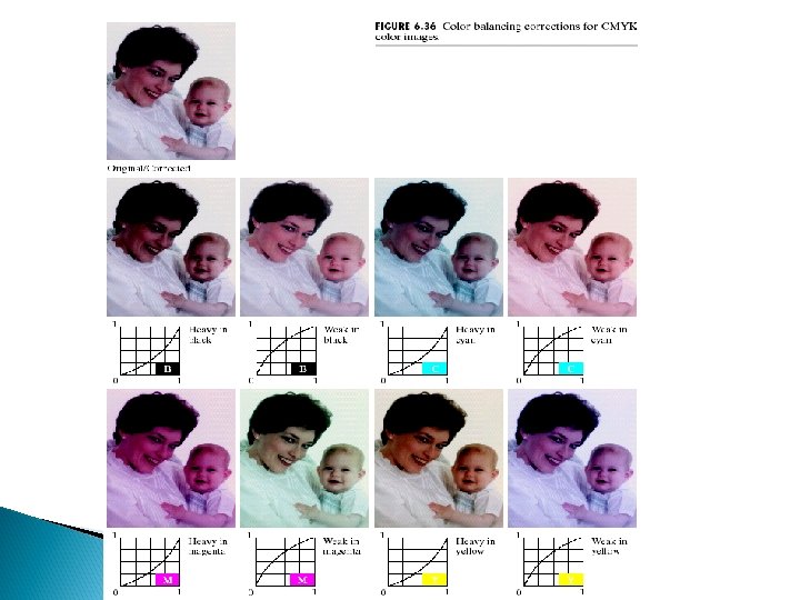
6. 5. 4 Tone and color correction ◦ Tonal range of an image (Key type)-refers to its general distribution of color intensities High-key image is concentrated at high intensities Low-key image are located at low intensities ◦ It is desirable to distribute the intensities of a color image equally between the highlight and shadow area ◦ Modifying tones normally are selected interactively ◦ Operation : adjust the images’ brightness and contrast over a suitable range of intensities In RGB and CMYK: map all three components In HIS : only intensity component is modified

Chapter 6 Color Image Processing

Color imbalance—analyzing with color spectrometer ◦ color wheel can be used to predict how one component will affect another ◦ The perception of one color is affected by its surrounding colors ◦ The portions of any color can be increased by decreasing the amount of the opposite ◦ Transformation functions required for correcting the images (Fig. 6. 36)

6. 5. 5 Histogram processing ◦ The gray-level processing can be applied to color images in an automatic way ◦ Produce an image with a uniform histogram of intensity values ◦ To histogram equalize the components of a color image individually is unwise (results in erroneous color) ◦ A more logical approach : spread the color intensities uniformly (use HSI space), leaving the colors themselves unchanged

Chapter 6 Color Image Processing

6. 6 smoothing and sharpening Instead of scalar gray-level values deal with vectors 6. 6. 1 Color image smoothing (Eq. 6. 6 -1 and 6. 6 -2) ◦ can be carried out on a per-color-plane basis ◦ smooth only the intensity component of the HSI representation and convert the processed result to an RGB image for display 6. 6. 2 Color image sharpening ◦ Laplacian of vector c: in RGB, and in I Component of HSI

Chapter 6 Color Image Processing

Chapter 6 Color Image Processing

Chapter 6 Color Image Processing

Chapter 6 Color Image Processing

6. 7 Color segmentation 6. 7. 1 Segmentation in HSI color space ◦ Carry out the segmentation process on individual planes(HSI) 1. color is conveniently represented in the Hue image 2. Saturation is used as a masking image 3. Intensity is used less frequently for segmentation

Chapter 6 Color Image Processing

6. 7. 2 Segmentation in RGB vector space ◦ Better results generally are obtained ◦ Obtain an estimate of the “average” color vector “a” ◦ Classify each RGB pixel as having a color in the specified range or not: by a measure of similarity (Euclidean distance)

Chapter 6 Color Image Processing

Distance measure with the covariance matrix D(z, a)=|| z-a|| ◦ if D(z, a) D 0 , Z is similar to a ◦ Implementing above is computationally expensive Distance measure with bounding box: Box dimension is proportional to the standard deviation of the sample along each of the axis Segment it by determining whether or not it is on the surface or inside the box —simpler computationally when compared to a spherical or elliptical enclosure

Chapter 6 Color Image Processing

6. 7. 3 Color edge detection ◦ Computing the gradient on individual images and then using the results to form a color image will lead to erroneous results (Fig. 6. 45) ◦ Individual based and vector-space based computing depend on accuracy or just detecting edges ◦ Extend the concept of a gradient from a scalar function to vector functions

Chapter 6 Color Image Processing

The def. of a gradient based on a vector Let r, g, and b be the unit vector along the R, G, and B axis of RGB color space and ◦ The direction of maximum rate of change of C(x, y) is given by angle ◦ The value of the rate of changes at (x, y) in the direction is given by ◦ ◦ gxx=u. u, gyy=v. v, gxy=u. v

Chapter 6 Color Image Processing

Chapter 6 Color Image Processing

6. 8 The noise in color images

Chapter 6 Color Image Processing

Chapter 6 Color Image Processing