AudioVisual Speech Recognition Audio Noise Video Noise and

Audio-Visual Speech Recognition: Audio Noise, Video Noise, and Pronunciation Variability Mark Hasegawa-Johnson Electrical and Computer Engineering

Audio-Visual Speech Recognition 1) Video Noise 1) Graphical Methods: Manifold Estimation 2) Local Graph Discriminant Features 2) Audio Noise 1) Beam-Form, Post-Filter, and Low-SNR VAD 3) Pronunciation Variability 1) Graphical Methods: Dynamic Bayesian Network 2) An Articulatory-Feature Model for Audio-Visual Speech Recognition

I. Video Noise 1) Graphical Methods: Manifold Estimation 2) Local Graph Discriminant Features 2) Audio Noise 1) Beam-Form, Post-Filter, and Low-SNR VAD 3) Pronunciation Variability 1) Graphical Methods: Dynamic Bayesian Network 2) An Articulatory-Feature Model for Audio-Visual Speech Recognition

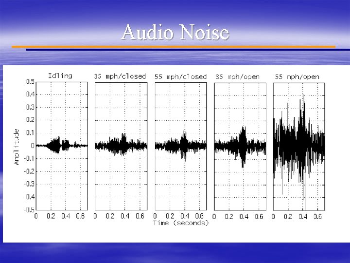
AVICAR Database ● ● ● AVICAR = Audio-Visual In a CAR 100 Talkers 4 Cameras, 7 Microphones 5 noise conditions: Engine idling, 35 mph with windows open, 55 mph with windows open Three types of utterances: – Digits & Phone numbers, for training and testing phonenumber recognizers – TIMIT sentences, for training and testing large vocabulary speech recognition – Isolated Letters, to test the use of video for an acoustically hard recognition problem

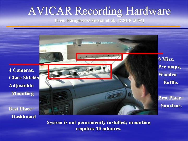
AVICAR Recording Hardware (Lee, Hasegawa-Johnson et al. , ICSLP 2004) 8 Mics, Pre-amps, Wooden Baffle. 4 Cameras, Glare Shields, Adjustable Mounting Best Place= Dashboard Best Place= Sunvisor. System is not permanently installed; mounting requires 10 minutes.

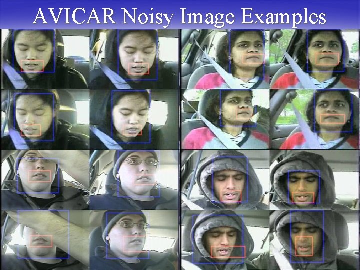
AVICAR Video Noise § Lighting: Many different angles, many types of weather § Interlace: 30 fps NTSC encoding used to transmit data from camera to digital video tape § Facial Features: – Hair – Skin – Clothing – Obstructions

AVICAR Noisy Image Examples

Related Problem: Dimensionality § Dimension of the raw grayscale lip rectangle: 30 x 200=6000 pixels § Dimension of the DCT of the lip rectangle: 30 x 200=6000 dimensions § Smallest truncated DCT that allows a human viewer to recognize lip shapes (Hasegawa-Johnson, informal experiments): 25 x 25=625 dimensions § Truncated DCT typically used in AVSR: 4 x 4=16 dimensions § Dimension of “geometric lip features” that allow high-accuracy AVSR (e. g. , Chu and Huang, 2000): 3 dimensions (lip height, lip width, vertical assymmetry)

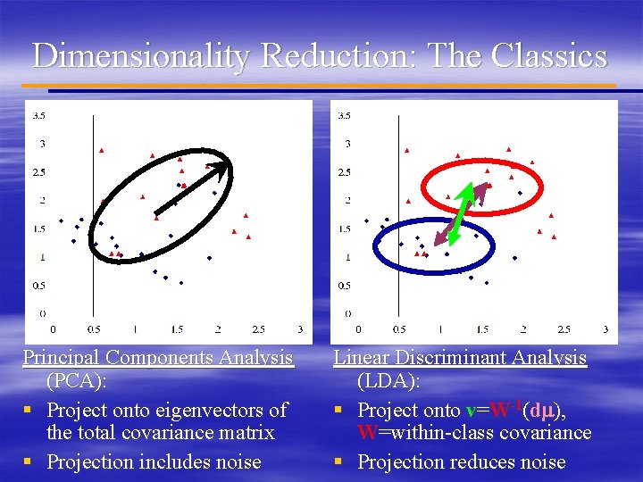
Dimensionality Reduction: The Classics Principal Components Analysis (PCA): § Project onto eigenvectors of the total covariance matrix § Projection includes noise Linear Discriminant Analysis (LDA): § Project onto v=W-1(dm), W=within-class covariance § Projection reduces noise

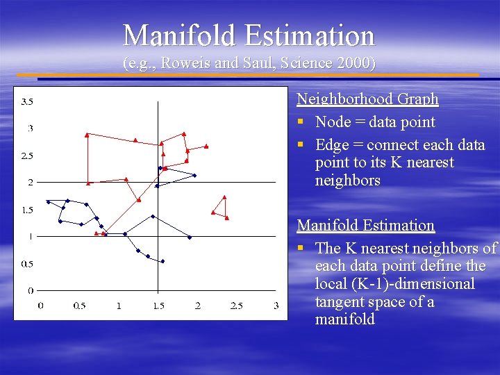
Manifold Estimation (e. g. , Roweis and Saul, Science 2000) Neighborhood Graph § Node = data point § Edge = connect each data point to its K nearest neighbors Manifold Estimation § The K nearest neighbors of each data point define the local (K-1)-dimensional tangent space of a manifold

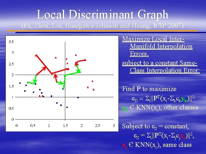
Local Discriminant Graph (Fu, Zhou, Liu, Hasegawa-Johnson and Huang, ICIP 2007) Maximize Local Inter. Manifold Interpolation Errors, subject to a constant Same. Class Interpolation Error: Find P to maximize e. D = Si||PT(xi-Skckyk)||2, yk Є KNN(xi), other classes Subject to e. S = constant, e. S = Si||PT(xi-Sjcjxj)||2, xj Є KNN(xi), same class

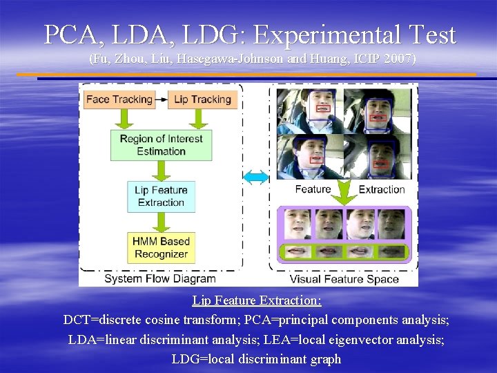
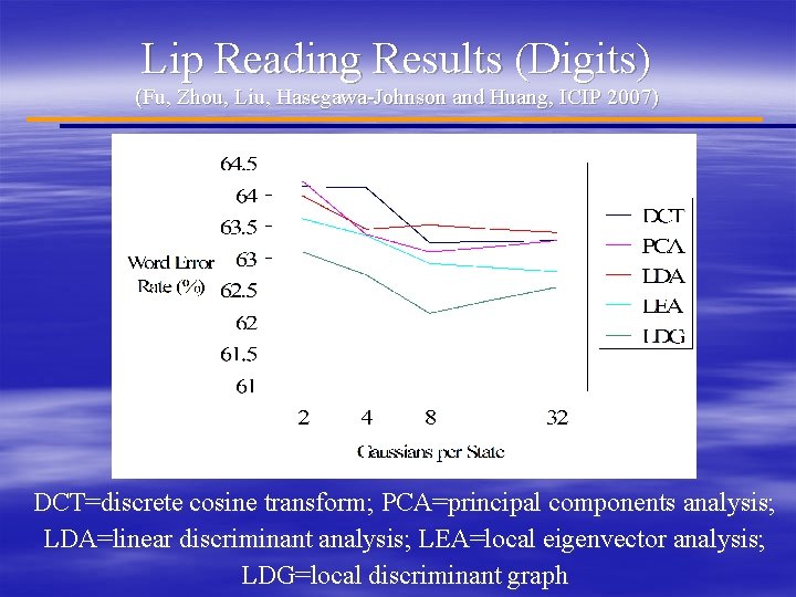
PCA, LDG: Experimental Test (Fu, Zhou, Liu, Hasegawa-Johnson and Huang, ICIP 2007) Lip Feature Extraction: DCT=discrete cosine transform; PCA=principal components analysis; LDA=linear discriminant analysis; LEA=local eigenvector analysis; LDG=local discriminant graph

Lip Reading Results (Digits) (Fu, Zhou, Liu, Hasegawa-Johnson and Huang, ICIP 2007) DCT=discrete cosine transform; PCA=principal components analysis; LDA=linear discriminant analysis; LEA=local eigenvector analysis; LDG=local discriminant graph

II. Audio Noise 1) Video Noise 1) Graphical Methods: Manifold Estimation 2) Local Graph Discriminant Features 2) Audio Noise 1) Beam-Form, Post-Filter, and Low-SNR VAD 3) Pronunciation Variability 1) Graphical Methods: Dynamic Bayesian Network 2) An Articulatory-Feature Model for Audio-Visual Speech Recognition

Audio Noise

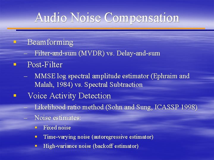
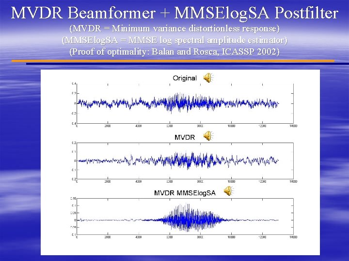
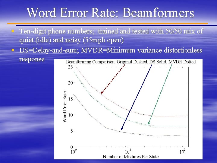
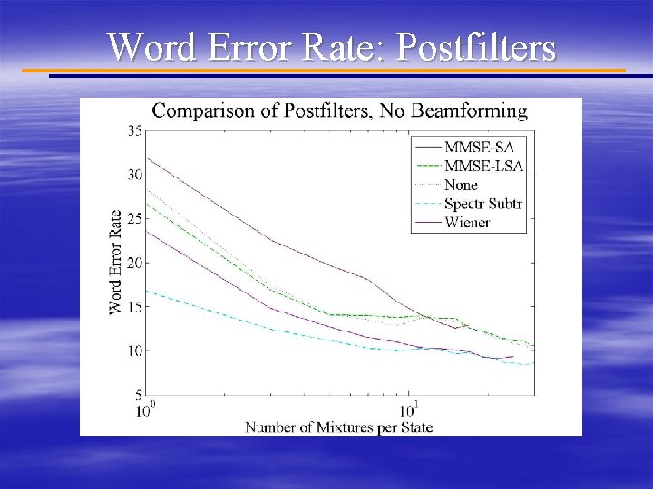
Audio Noise Compensation § Beamforming – Filter-and-sum (MVDR) vs. Delay-and-sum § Post-Filter – MMSE log spectral amplitude estimator (Ephraim and Malah, 1984) vs. Spectral Subtraction § Voice Activity Detection – Likelihood ratio method (Sohn and Sung, ICASSP 1998) – Noise estimates: § Fixed noise § Time-varying noise (autoregressive estimator) § High-variance noise (backoff estimator)

MVDR Beamformer + MMSElog. SA Postfilter (MVDR = Minimum variance distortionless response) (MMSElog. SA = MMSE log spectral amplitude estimator) (Proof of optimality: Balan and Rosca, ICASSP 2002)

Word Error Rate: Beamformers § Ten-digit phone numbers; trained and tested with 50/50 mix of quiet (idle) and noisy (55 mph open) § DS=Delay-and-sum; MVDR=Minimum variance distortionless response

Word Error Rate: Postfilters

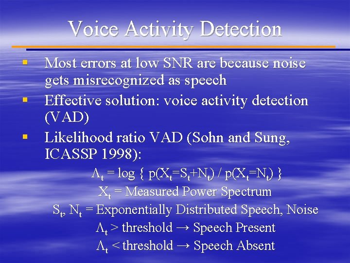
Voice Activity Detection § Most errors at low SNR are because noise gets misrecognized as speech § Effective solution: voice activity detection (VAD) § Likelihood ratio VAD (Sohn and Sung, ICASSP 1998): Lt = log { p(Xt=St+Nt) / p(Xt=Nt) } Xt = Measured Power Spectrum St, Nt = Exponentially Distributed Speech, Noise Lt > threshold → Speech Present Lt < threshold → Speech Absent

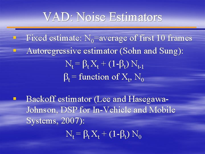
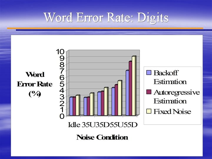
VAD: Noise Estimators § Fixed estimate: N 0=average of first 10 frames § Autoregressive estimator (Sohn and Sung): Nt = bt Xt + (1 -bt) Nt-1 bt = function of Xt, N 0 § Backoff estimator (Lee and Hasegawa. Johnson, DSP for In-Vehicle and Mobile Systems, 2007): Nt = bt Xt + (1 -bt) N 0

Word Error Rate: Digits

III. Pronunciation Variability 1) Video Noise 1) Graphical Methods: Manifold Estimation 2) Local Graph Discriminant Features 2) Audio Noise 1) Beam-Form, Post-Filter, and Low-SNR VAD 3) Pronunciation Variability 1) Graphical Methods: Dynamic Bayesian Network 2) An Articulatory-Feature Model for Audio-Visual Speech Recognition

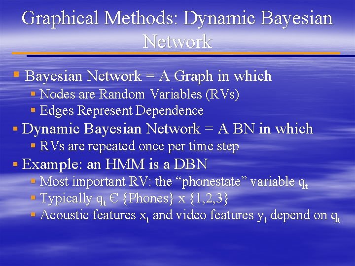
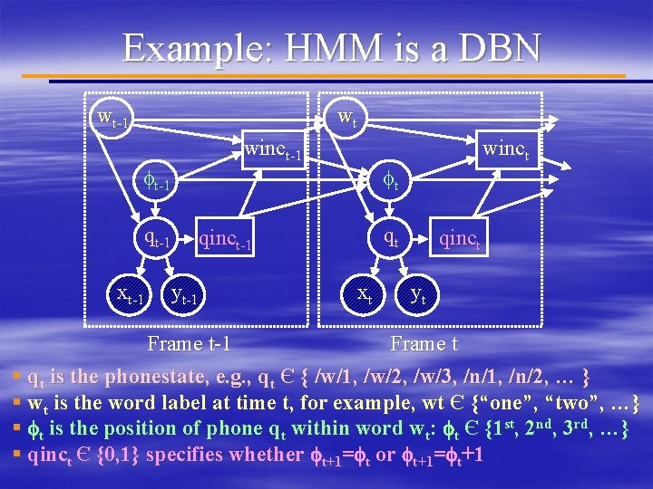
Graphical Methods: Dynamic Bayesian Network § Bayesian Network = A Graph in which § Nodes are Random Variables (RVs) § Edges Represent Dependence § Dynamic Bayesian Network = A BN in which § RVs are repeated once per time step § Example: an HMM is a DBN § Most important RV: the “phonestate” variable qt § Typically qt Є {Phones} x {1, 2, 3} § Acoustic features xt and video features yt depend on qt

Example: HMM is a DBN wt-1 wt winct-1 ft-1 qt-1 xt-1 ft qt qinct-1 yt-1 winct xt qinct yt Frame t-1 Frame t § qt is the phonestate, e. g. , qt Є { /w/1, /w/2, /w/3, /n/1, /n/2, … } § wt is the word label at time t, for example, wt Є {“one”, “two”, …} § ft is the position of phone qt within word wt: ft Є {1 st, 2 nd, 3 rd, …} § qinct Є {0, 1} specifies whether ft+1=ft or ft+1=ft+1

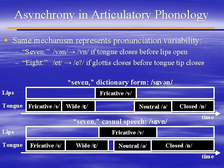
Pronunciation Variability § Even when reading phone numbers, talkers “blend” articulations. § For example: “seven eight: ” /sevәnet/→ /sevne? / § As speech gets less formal, pronunciation variability gets worse, e. g. , worse in a car than in the lab; worse in conversation than in read speech

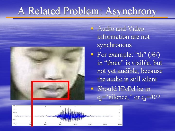
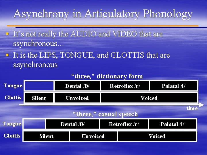
A Related Problem: Asynchrony § Audio and Video information are not synchronous § For example: “th” (/q/) in “three” is visible, but not yet audible, because the audio is still silent § Should HMM be in qt=“silence, ” or qt=/q/?

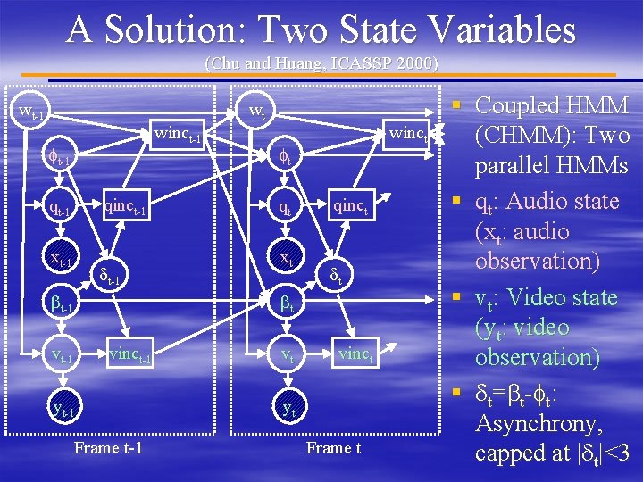
A Solution: Two State Variables (Chu and Huang, ICASSP 2000) wt-1 winct-1 ft-1 qinct-1 qt-1 xt-1 dt-1 bt-1 vt-1 wt winct ft qt xt qinct dt bt vinct-1 yt-1 Frame t-1 vt vinct yt Frame t § Coupled HMM (CHMM): Two parallel HMMs § qt: Audio state (xt: audio observation) § vt: Video state (yt: video observation) § d t = b t -f t : Asynchrony, capped at |dt|<3

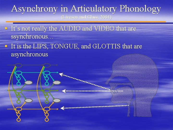
Asynchrony in Articulatory Phonology (Livescu and Glass, 2004) § It’s not really the AUDIO and VIDEO that are ssynchronous… § It is the LIPS, TONGUE, and GLOTTIS that are asynchronous word ind 1 U 1 sync 1, 2 S 1 ind 2 U 2 sync 2, 3 S 2 ind 3 U 3 S 3

Asynchrony in Articulatory Phonology § It’s not really the AUDIO and VIDEO that are ssynchronous… § It is the LIPS, TONGUE, and GLOTTIS that are asynchronous “three, ” dictionary form Tongue Glottis Dental /q/ Silent Retroflex /r/ Unvoiced Palatal /i/ Voiced time “three, ” casual speech Tongue Glottis Dental /q/ Silent Unvoiced Retroflex /r/ Palatal /i/ Voiced

Asynchrony in Articulatory Phonology § Same mechanism represents pronunciation variability: – “Seven: ” /vәn/→ /vn/ if tongue closes before lips open – “Eight: ” /et/ → /e? / if glottis closes before tongue tip closes “seven, ” dictionary form: /sevәn/ Lips Fricative /v/ Tongue Fricative /s/ Wide /e/ Neutral /ә/ Closed /n/ “seven, ” casual speech: /sevn/ Lips Tongue time Fricative /v/ Fricative /s/ Wide /e/ Neutral /ә/ Closed /n/ time

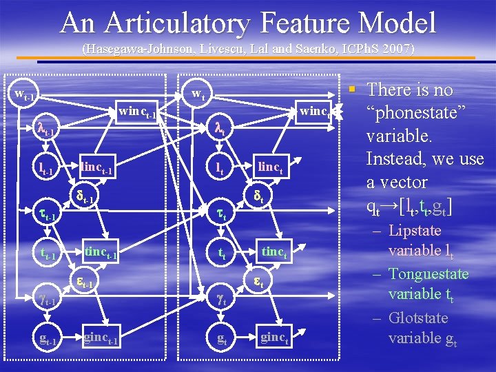
An Articulatory Feature Model (Hasegawa-Johnson, Livescu, Lal and Saenko, ICPh. S 2007) wt-1 winct-1 lt-1 tt-1 gt-1 linct-1 dt-1 tinct-1 et-1 ginct-1 wt winct lt lt tt tt gt gt linct dt tinct et ginct § There is no “phonestate” variable. Instead, we use a vector qt→[lt, tt, gt] – Lipstate variable lt – Tonguestate variable tt – Glotstate variable gt

Experimental Test (Hasegawa-Johnson, Livescu, Lal and Saenko, ICPh. S 2007) § Training and test data: CUAVE corpus – Patterson, Gurbuz, Turfecki and Gowdy, ICASSP 2002 – 169 utterances used, 10 digits each, silence between words – Recorded without Audio or Video noise (studio lighting; silent bkgd) § Audio prepared by Kate Saenko at MIT – NOISEX speech babble added at various SNRs – MFCC+d+dd feature vectors, 10 ms frames § Video prepared by Amar Subramanya at UW – Feature vector = DCT of lip rectangle – Upsampled from 33 ms frames to 10 ms frames § Experimental Condition: Train-Test Mismatch – Training on clean data – Audio/video weights tuned on noise-specific dev sets – Language model: uniform (all words equal probability), constrained to have the right number of words per utterance

Experimental Questions (Hasegawa-Johnson, Livescu, Lal and Saenko, ICPh. S 2007) 1) Does Video reduce word error rate? 2) Does Audio-Video Asynchrony reduce word error rate? 3) Should asynchrony be represented as 1) Audio-Video Asynchrony (CHMM), or 2) Lips-Tongue-Glottis Asynchrony (AFM) 4) Is it better to use only CHMM, only AFM, or a combination of both methods?

Results, part 1: Should we use video? Answer: YES. Audio-Visual WER < Single-stream WER

Results, part 2: Are Audio and Video be asynchronous? Answer: YES. Async WER < Sync WER.

Results, part 3: Should we use CHMM or AFM? Answer: DOESN’T MATTER! WERs are equal.

Results, part 4: Should we combine systems? Answer: YES. Best is AFM+CH 1+CH 2 ROVER

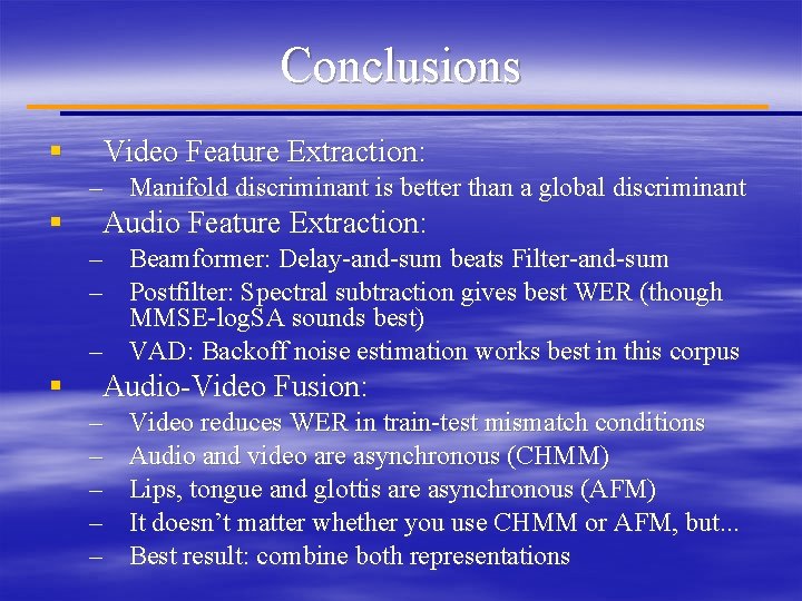
Conclusions § Video Feature Extraction: – Manifold discriminant is better than a global discriminant § Audio Feature Extraction: – Beamformer: Delay-and-sum beats Filter-and-sum – Postfilter: Spectral subtraction gives best WER (though MMSE-log. SA sounds best) – VAD: Backoff noise estimation works best in this corpus § Audio-Video Fusion: – – – Video reduces WER in train-test mismatch conditions Audio and video are asynchronous (CHMM) Lips, tongue and glottis are asynchronous (AFM) It doesn’t matter whether you use CHMM or AFM, but. . . Best result: combine both representations