Approximate computation and implicit regularization for very largescale

Approximate computation and implicit regularization for very large-scale data analysis Michael W. Mahoney Stanford University May 2012 (For more info, see: http: //cs. stanford. edu/people/mmahoney)

Algorithmic vs. Statistical Perspectives Lambert (2000); Mahoney “Algorithmic and Statistical Perspectives on Large-Scale Data Analysis” (2010) Computer Scientists • Data: are a record of everything that happened. • Goal: process the data to find interesting patterns and associations. • Methodology: Develop approximation algorithms under different models of data access since the goal is typically computationally hard. Statisticians (and Natural Scientists, etc) • Data: are a particular random instantiation of an underlying process describing unobserved patterns in the world. • Goal: is to extract information about the world from noisy data. • Methodology: Make inferences (perhaps about unseen events) by positing a model that describes the random variability of the data around the deterministic model.

Perspectives are NOT incompatible • Statistical/probabilistic ideas are central to recent work on developing improved randomized algorithms for matrix problems. • Intractable optimization problems on graphs/networks yield to approximation when assumptions are made about network participants. • In boosting (a statistical technique that fits an additive model by minimizing an objective function with a method such as gradient descent), the computation parameter (i. e. , the number of iterations) also serves as a regularization parameter.

But they are VERY different paradigms Statistics, natural sciences, scientific computing, etc: • Problems often involve computation, but the study of computation per se is secondary • Only makes sense to develop algorithms for well-posed* problems • First, write down a model, and think about computation later Computer science: • Easier to study computation per se in discrete settings, e. g. , Turing machines, logic, complexity classes • Theory of algorithms divorces computation from data • First, run a fast algorithm, and ask what it means later *Solution exists, is unique, and varies continuously with input data

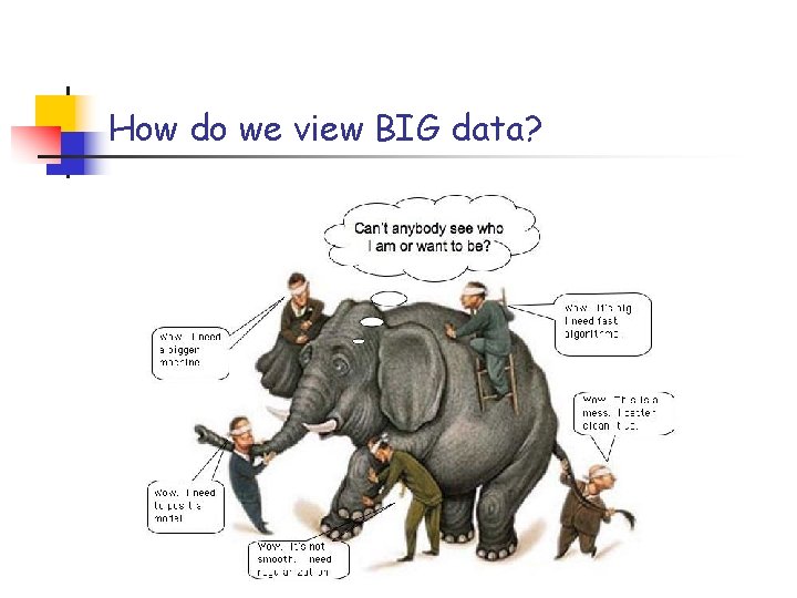
How do we view BIG data?

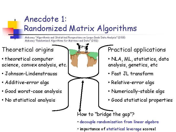
Anecdote 1: Randomized Matrix Algorithms Mahoney “Algorithmic and Statistical Perspectives on Large-Scale Data Analysis” (2010) Mahoney “Randomized Algorithms for Matrices and Data” (2011) Theoretical origins Practical applications • theoretical computer science, convex analysis, etc. • NLA, ML, statistics, data analysis, genetics, etc • Johnson-Lindenstrauss • Fast JL transform • Additive-error algs • Relative-error algs • Good worst-case analysis • Numerically-stable algs • No statistical analysis • Good statistical properties How to “bridge the gap”? • decouple randomization from linear algebra • importance of statistical leverage scores!

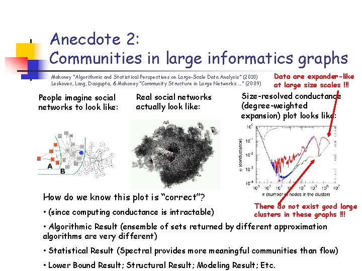
Anecdote 2: Communities in large informatics graphs Mahoney “Algorithmic and Statistical Perspectives on Large-Scale Data Analysis” (2010) Leskovec, Lang, Dasgupta, & Mahoney “Community Structure in Large Networks. . . ” (2009) People imagine social networks to look like: Real social networks actually look like: How do we know this plot is “correct”? • (since computing conductance is intractable) Data are expander-like at large size scales !!! Size-resolved conductance (degree-weighted expansion) plot looks like: There do not exist good large clusters in these graphs !!! • Algorithmic Result (ensemble of sets returned by different approximation algorithms are very different) • Statistical Result (Spectral provides more meaningful communities than flow) • Lower Bound Result; Structural Result; Modeling Result; Etc.

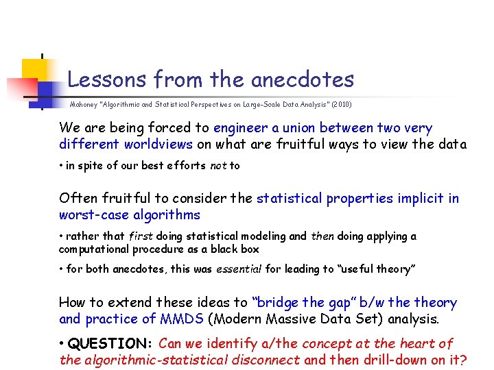
Lessons from the anecdotes Mahoney “Algorithmic and Statistical Perspectives on Large-Scale Data Analysis” (2010) We are being forced to engineer a union between two very different worldviews on what are fruitful ways to view the data • in spite of our best efforts not to Often fruitful to consider the statistical properties implicit in worst-case algorithms • rather that first doing statistical modeling and then doing applying a computational procedure as a black box • for both anecdotes, this was essential for leading to “useful theory” How to extend these ideas to “bridge the gap” b/w theory and practice of MMDS (Modern Massive Data Set) analysis. • QUESTION: Can we identify a/the concept at the heart of the algorithmic-statistical disconnect and then drill-down on it?

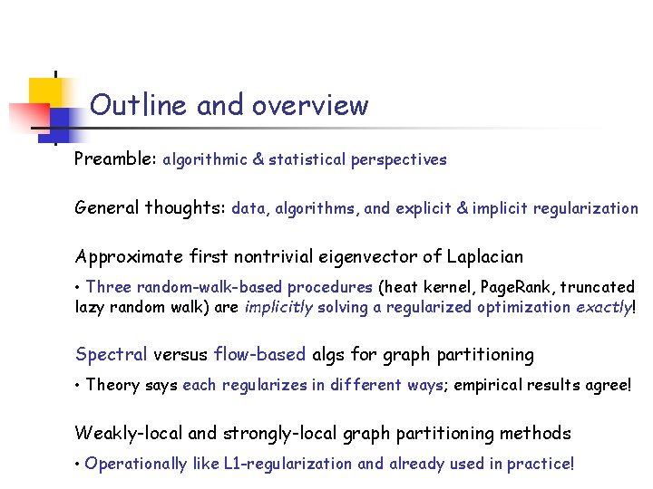
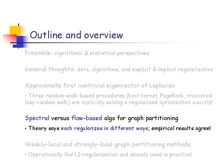
Outline and overview Preamble: algorithmic & statistical perspectives General thoughts: data, algorithms, and explicit & implicit regularization Approximate first nontrivial eigenvector of Laplacian • Three random-walk-based procedures (heat kernel, Page. Rank, truncated lazy random walk) are implicitly solving a regularized optimization exactly! Spectral versus flow-based algs for graph partitioning • Theory says each regularizes in different ways; empirical results agree! Weakly-local and strongly-local graph partitioning methods • Operationally like L 1 -regularization and already used in practice!

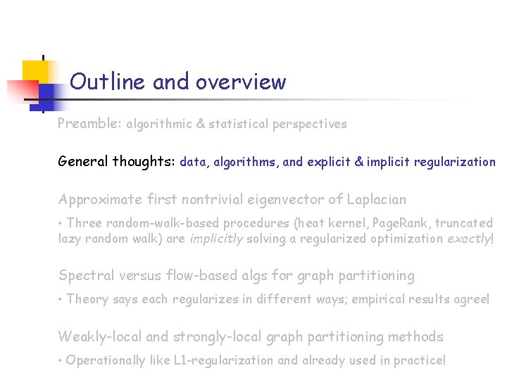
Outline and overview Preamble: algorithmic & statistical perspectives General thoughts: data, algorithms, and explicit & implicit regularization Approximate first nontrivial eigenvector of Laplacian • Three random-walk-based procedures (heat kernel, Page. Rank, truncated lazy random walk) are implicitly solving a regularized optimization exactly! Spectral versus flow-based algs for graph partitioning • Theory says each regularizes in different ways; empirical results agree! Weakly-local and strongly-local graph partitioning methods • Operationally like L 1 -regularization and already used in practice!

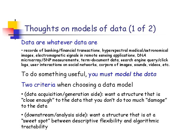
Thoughts on models of data (1 of 2) Data are whatever data are • records of banking/financial transactions, hyperspectral medical/astronomical images, electromagnetic signals in remote sensing applications, DNA microarray/SNP measurements, term-document data, search engine query/click logs, user interactions on social networks, corpora of images, sounds, videos, etc. To do something useful, you must model the data Two criteria when choosing a data model • (data acquisition/generation side): want a structure that is “close enough” to the data that you don’t do too much “damage” to the data • (downstream/analysis side): want a structure that is at a “sweet spot” between descriptive flexibility and algorithmic tractability

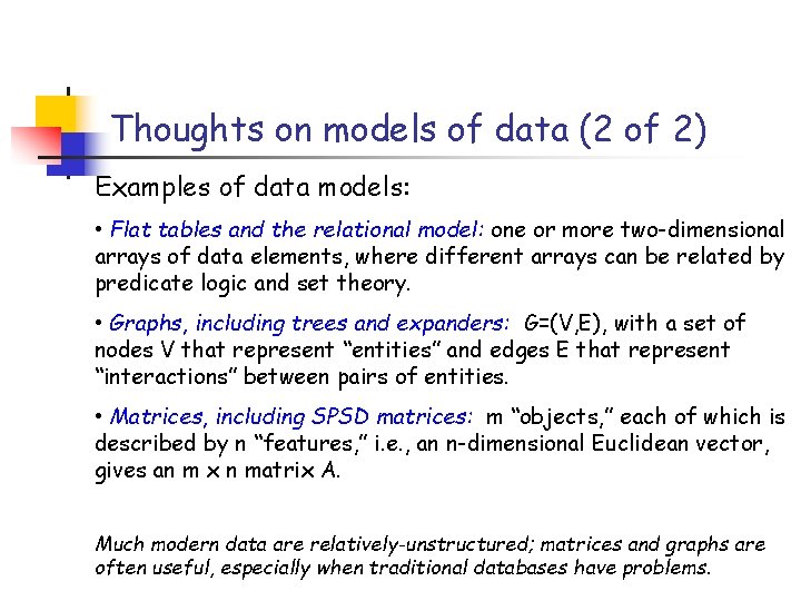
Thoughts on models of data (2 of 2) Examples of data models: • Flat tables and the relational model: one or more two-dimensional arrays of data elements, where different arrays can be related by predicate logic and set theory. • Graphs, including trees and expanders: G=(V, E), with a set of nodes V that represent “entities” and edges E that represent “interactions” between pairs of entities. • Matrices, including SPSD matrices: m “objects, ” each of which is described by n “features, ” i. e. , an n-dimensional Euclidean vector, gives an m x n matrix A. Much modern data are relatively-unstructured; matrices and graphs are often useful, especially when traditional databases have problems.

Relationship b/w algorithms and data (1 of 3) Before the digital computer: • Natural sciences rich source of problems, statistical methods developed to solve those problems • Very important notion: well-posed (well-conditioned) problem: solution exists, is unique, and is continuous w. r. t. problem parameters • Simply doesn’t make sense to solve ill-posed problems Advent of the digital computer: • Split in (yet-to-be-formed field of) “Computer Science” • Based on application (scientific/numerical computing vs. business/consumer applications) as well as tools (continuous math vs. discrete math) • Two very different perspectives on relationship b/w algorithms and data

Relationship b/w algorithms and data (2 of 3) Two-step approach for “numerical” problems • Is problem well-posed/well-conditioned? • If no, replace it with a well-posed problem. (Regularization!) • If yes, design a stable algorithm. View Algorithm A as a function f • Given x, it tries to compute y but actually computes y* • Forward error: Δy=y*-y • Backward error: smallest Δx s. t. f(x+Δx) = y* • Forward error ≤ Backward error * condition number • Backward-stable algorithm provides accurate solution to well-posed problem!

Relationship b/w algorithms and data (3 of 3) One-step approach for study of computation, per se • Concept of computability captured by 3 seemingly-different discrete processes (recursion theory, λ-calculus, Turing machine) • Computable functions have internal structure (P vs. NP, NP-hardness, etc. ) • Problems of practical interest are “intractable” (e. g. , NP-hard vs. poly(n), or O(n 3) vs. O(n log n)) Modern Theory of Approximation Algorithms • provides forward-error bounds for worst-cast input • worst case in two senses: (1) for all possible input & (2) i. t. o. relativelysimple complexity measures, but independent of “structural parameters” • get bounds by “relaxations” of IP to LP/SDP/etc. , i. e. , a “nicer” place

Statistical regularization (1 of 3) Regularization in statistics, ML, and data analysis • arose in integral equation theory to “solve” ill-posed problems • computes a better or more “robust” solution, so better inference • involves making (explicitly or implicitly) assumptions about data • provides a trade-off between “solution quality” versus “solution niceness” • often, heuristic approximation procedures have regularization properties as a “side effect” • lies at the heart of the disconnect between the “algorithmic perspective” and the “statistical perspective”

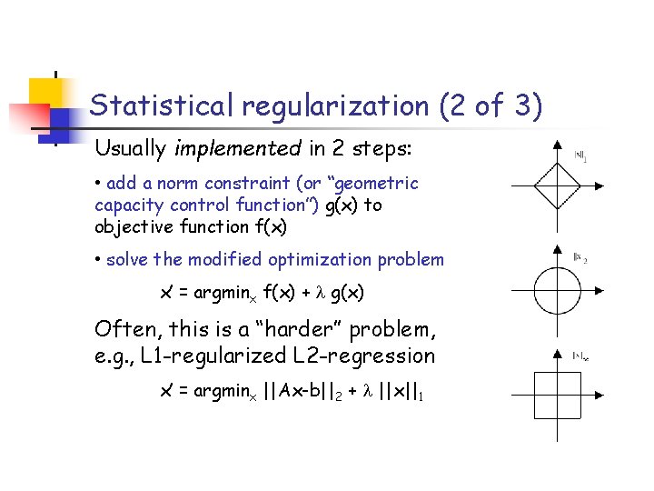
Statistical regularization (2 of 3) Usually implemented in 2 steps: • add a norm constraint (or “geometric capacity control function”) g(x) to objective function f(x) • solve the modified optimization problem x’ = argminx f(x) + g(x) Often, this is a “harder” problem, e. g. , L 1 -regularized L 2 -regression x’ = argminx ||Ax-b||2 + ||x||1

Statistical regularization (3 of 3) Regularization is often observed as a side-effect or byproduct of other design decisions • “binning, ” “pruning, ” etc. • “truncating” small entries to zero, “early stopping” of iterations • approximation algorithms and heuristic approximations engineers do to implement algorithms in large-scale systems BIG question: Can we formalize the notion that/when approximate computation can implicitly lead to “better” or “more regular” solutions than exact computation?

Outline and overview Preamble: algorithmic & statistical perspectives General thoughts: data, algorithms, and explicit & implicit regularization Approximate first nontrivial eigenvector of Laplacian • Three random-walk-based procedures (heat kernel, Page. Rank, truncated lazy random walk) are implicitly solving a regularized optimization exactly! Spectral versus flow-based algs for graph partitioning • Theory says each regularizes in different ways; empirical results agree! Weakly-local and strongly-local graph partitioning methods • Operationally like L 1 -regularization and already used in practice!

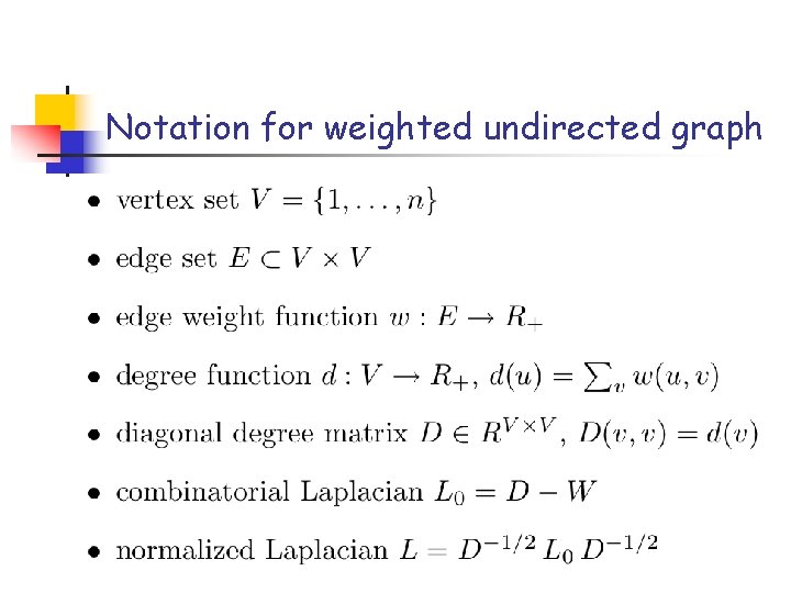
Notation for weighted undirected graph

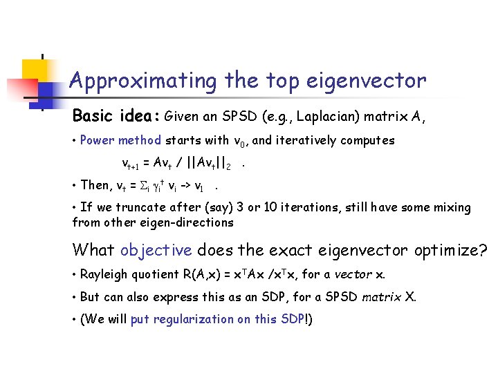
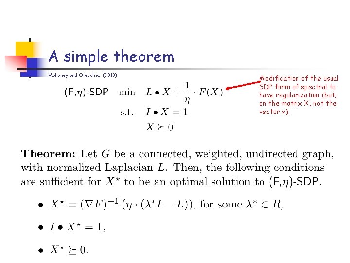
Approximating the top eigenvector Basic idea: Given an SPSD (e. g. , Laplacian) matrix A, • Power method starts with v 0, and iteratively computes vt+1 = Avt / ||Avt||2. • Then, vt = i it vi -> v 1. • If we truncate after (say) 3 or 10 iterations, still have some mixing from other eigen-directions What objective does the exact eigenvector optimize? • Rayleigh quotient R(A, x) = x. TAx /x. Tx, for a vector x. • But can also express this as an SDP, for a SPSD matrix X. • (We will put regularization on this SDP!)

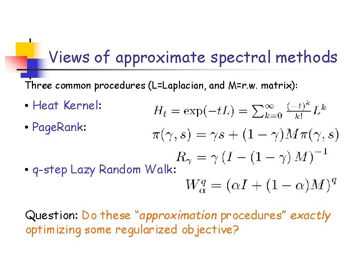
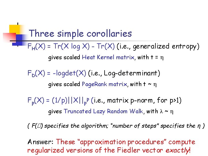
Views of approximate spectral methods Three common procedures (L=Laplacian, and M=r. w. matrix): • Heat Kernel: • Page. Rank: • q-step Lazy Random Walk: Question: Do these “approximation procedures” exactly optimizing some regularized objective?

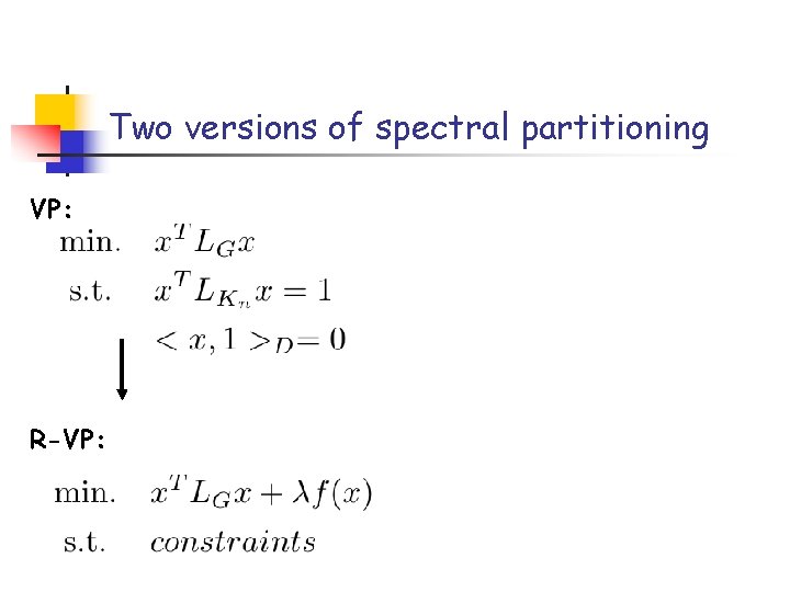
Two versions of spectral partitioning VP: R-VP:

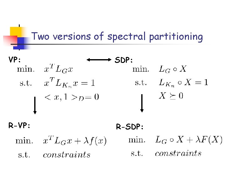
Two versions of spectral partitioning VP: SDP: R-VP: R-SDP:

A simple theorem Mahoney and Orecchia (2010) Modification of the usual SDP form of spectral to have regularization (but, on the matrix X, not the vector x).

Three simple corollaries FH(X) = Tr(X log X) - Tr(X) (i. e. , generalized entropy) gives scaled Heat Kernel matrix, with t = FD(X) = -logdet(X) (i. e. , Log-determinant) gives scaled Page. Rank matrix, with t ~ Fp(X) = (1/p)||X||pp (i. e. , matrix p-norm, for p>1) gives Truncated Lazy Random Walk, with ~ ( F(�) specifies the algorithm; “number of steps” specifies the η ) Answer: These “approximation procedures” compute regularized versions of the Fiedler vector exactly!

Outline and overview Preamble: algorithmic & statistical perspectives General thoughts: data, algorithms, and explicit & implicit regularization Approximate first nontrivial eigenvector of Laplacian • Three random-walk-based procedures (heat kernel, Page. Rank, truncated lazy random walk) are implicitly solving a regularized optimization exactly! Spectral versus flow-based algs for graph partitioning • Theory says each regularizes in different ways; empirical results agree! Weakly-local and strongly-local graph partitioning methods • Operationally like L 1 -regularization and already used in practice!

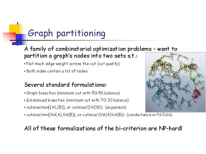
Graph partitioning A family of combinatorial optimization problems - want to partition a graph’s nodes into two sets s. t. : • Not much edge weight across the cut (cut quality) • Both sides contain a lot of nodes Several standard formulations: • Graph bisection (minimum cut with 50 -50 balance) • -balanced bisection (minimum cut with 70 -30 balance) • cutsize/min{|A|, |B|}, or cutsize/(|A||B|) (expansion) • cutsize/min{Vol(A), Vol(B)}, or cutsize/(Vol(A)Vol(B)) (conductance or N-Cuts) All of these formalizations of the bi-criterion are NP-hard!

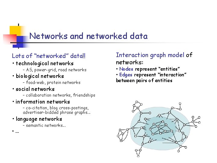
Networks and networked data Lots of “networked” data!! • technological networks – AS, power-grid, road networks • biological networks – food-web, protein networks • social networks – collaboration networks, friendships • information networks – co-citation, blog cross-postings, advertiser-bidded phrase graphs. . . • language networks • . . . – semantic networks. . . Interaction graph model of networks: • Nodes represent “entities” • Edges represent “interaction” between pairs of entities

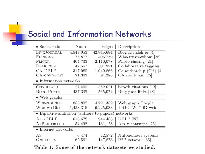
Social and Information Networks

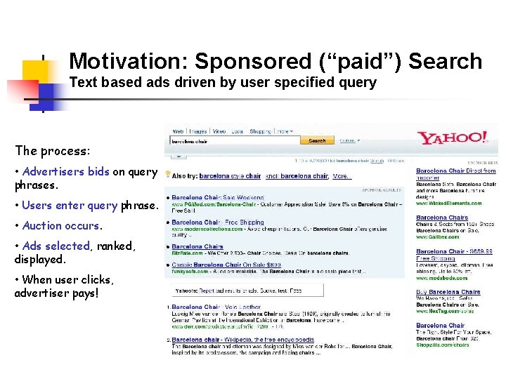
Motivation: Sponsored (“paid”) Search Text based ads driven by user specified query The process: • Advertisers bids on query phrases. • Users enter query phrase. • Auction occurs. • Ads selected, ranked, displayed. • When user clicks, advertiser pays!

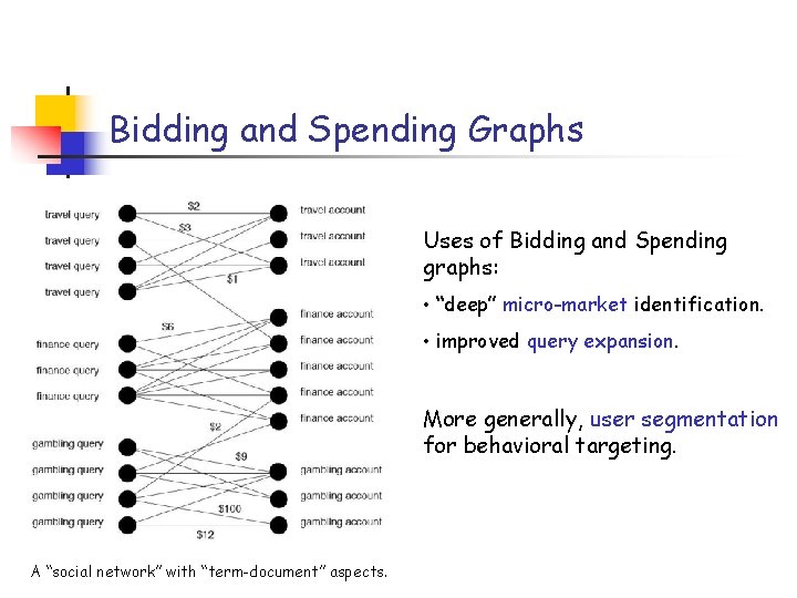
Bidding and Spending Graphs Uses of Bidding and Spending graphs: • “deep” micro-market identification. • improved query expansion. More generally, user segmentation for behavioral targeting. A “social network” with “term-document” aspects.

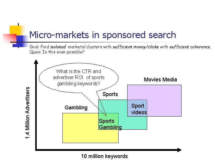
Micro-markets in sponsored search Goal: Find isolated markets/clusters with sufficient money/clicks with sufficient coherence. Ques: Is this even possible? 1. 4 Million Advertisers What is the CTR and advertiser ROI of sports gambling keywords? Movies Media Sports Sport videos Gambling Sports Gambling 10 million keywords

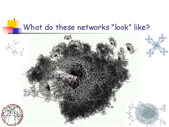
What do these networks “look” like?

The “lay of the land” Spectral methods* - compute eigenvectors of associated matrices Local improvement - easily get trapped in local minima, but can be used to clean up other cuts Multi-resolution - view (typically space-like graphs) at multiple size scales Flow-based methods* - single-commodity or multicommodity version of max-flow-min-cut ideas *Comes with strong underlying theory to guide heuristics.

Comparison of “spectral” versus “flow” Spectral: Flow: • Compute an eigenvector • Compute a LP • “Quadratic” worst-case bounds • O(log n) worst-case bounds • Worst-case achieved -- on “long • Worst-case achieved -- on stringy” graphs expanders • Worse-case is “local” property • Worst case is “global” property • Embeds you on a line (or Kn) • Embeds you in L 1 Two methods -- complementary strengths and weaknesses • What we compute is determined at least as much by as the approximation algorithm as by objective function.

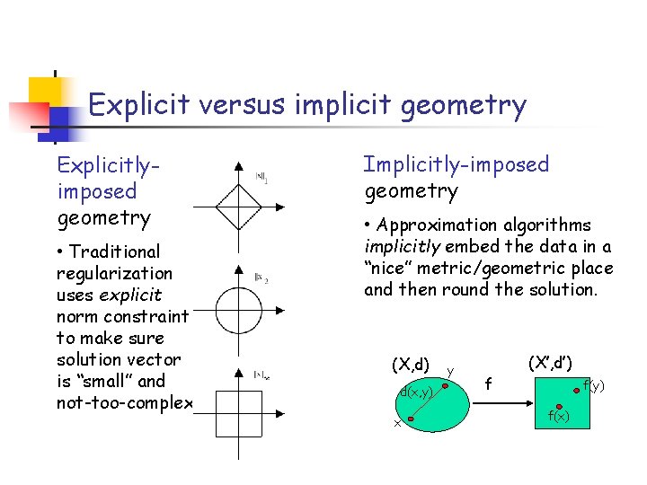
Explicit versus implicit geometry Explicitlyimposed geometry • Traditional regularization uses explicit norm constraint to make sure solution vector is “small” and not-too-complex Implicitly-imposed geometry • Approximation algorithms implicitly embed the data in a “nice” metric/geometric place and then round the solution. (X, d) d(x, y) x y f (X’, d’) f(y) f(x)

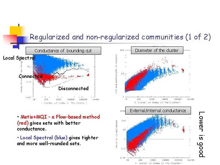
Regularized and non-regularized communities (1 of 2) Conductance of bounding cut Diameter of the cluster Local Spectral Connected Disconnected • Metis+MQI - a Flow-based method (red) gives sets with better conductance. • Local Spectral (blue) gives tighter and more well-rounded sets. Lower is good External/internal conductance

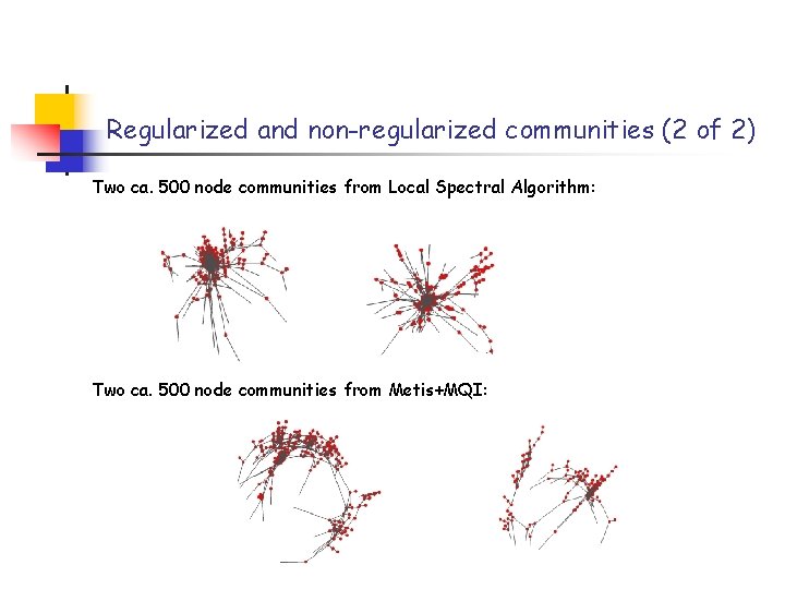
Regularized and non-regularized communities (2 of 2) Two ca. 500 node communities from Local Spectral Algorithm: Two ca. 500 node communities from Metis+MQI:

Outline and overview Preamble: algorithmic & statistical perspectives General thoughts: data, algorithms, and explicit & implicit regularization Approximate first nontrivial eigenvector of Laplacian • Three random-walk-based procedures (heat kernel, Page. Rank, truncated lazy random walk) are implicitly solving a regularized optimization exactly! Spectral versus flow-based algs for graph partitioning • Theory says each regularizes in different ways; empirical results agree! Weakly-local and strongly-local graph partitioning methods • Operationally like L 1 -regularization, and already used in practice!

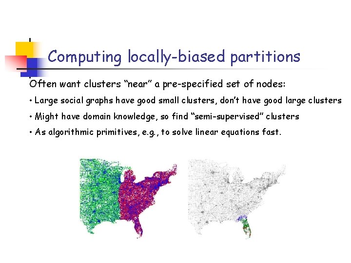
Computing locally-biased partitions Often want clusters “near” a pre-specified set of nodes: • Large social graphs have good small clusters, don’t have good large clusters • Might have domain knowledge, so find “semi-supervised” clusters • As algorithmic primitives, e. g. , to solve linear equations fast.

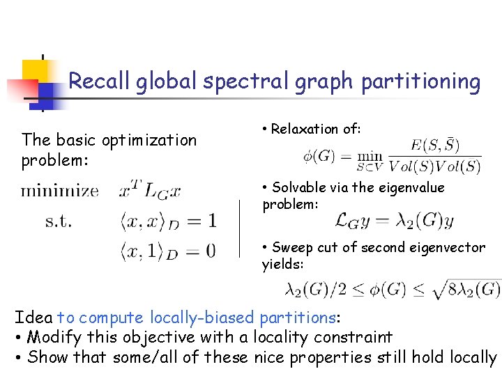
Recall global spectral graph partitioning The basic optimization problem: • Relaxation of: • Solvable via the eigenvalue problem: • Sweep cut of second eigenvector yields: Idea to compute locally-biased partitions: • Modify this objective with a locality constraint • Show that some/all of these nice properties still hold locally

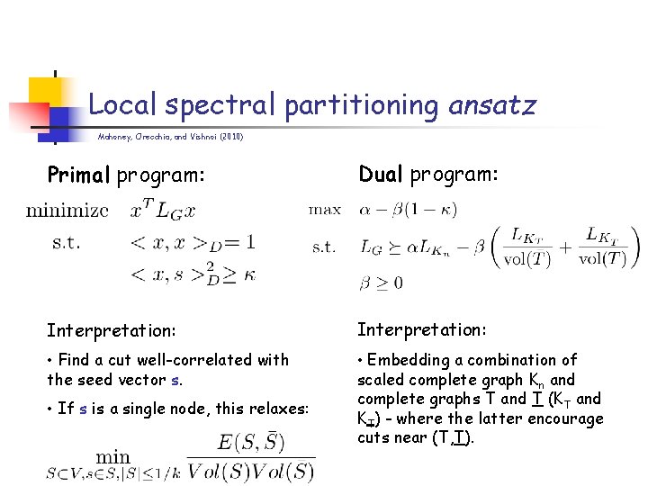
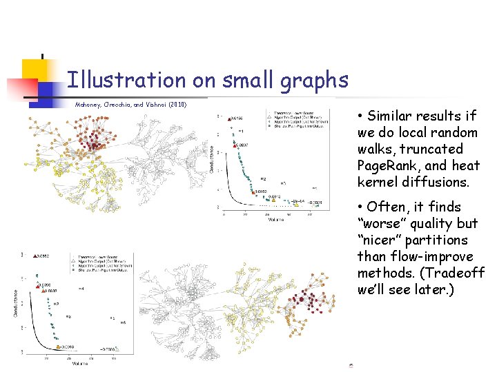
Local spectral partitioning ansatz Mahoney, Orecchia, and Vishnoi (2010) Primal program: Dual program: Interpretation: • Find a cut well-correlated with the seed vector s. • Embedding a combination of scaled complete graph Kn and complete graphs T and T (KT and KT) - where the latter encourage cuts near (T, T). • If s is a single node, this relaxes:

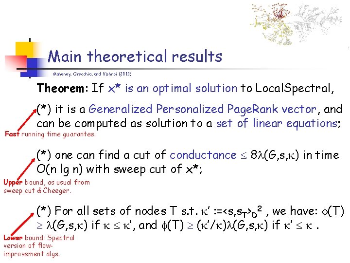
Main theoretical results Mahoney, Orecchia, and Vishnoi (2010) Theorem: If x* is an optimal solution to Local. Spectral, (*) it is a Generalized Personalized Page. Rank vector, and can be computed as solution to a set of linear equations; Fast running time guarantee. (*) one can find a cut of conductance 8 (G, s, ) in time O(n lg n) with sweep cut of x*; Upper bound, as usual from sweep cut & Cheeger. (*) For all sets of nodes T s. t. ’ : =<s, s. T>D 2 , we have: (T) (G, s, ) if ’, and (T) ( ’/ ) (G, s, ) if ’ . Lower bound: Spectral version of flowimprovement algs.

Illustration on small graphs Mahoney, Orecchia, and Vishnoi (2010) • Similar results if we do local random walks, truncated Page. Rank, and heat kernel diffusions. • Often, it finds “worse” quality but “nicer” partitions than flow-improve methods. (Tradeoff we’ll see later. )

A somewhat different approach Strongly-local spectral methods ST 04: truncated “local” random walks to compute locally-biased cut ACL 06: approximate locally-biased Page. Rank vector computations Chung 08: approximate heat-kernel computation to get a vector These are the diffusion-based procedures that we saw before except truncate/round/clip/push small things to zero starting with localized initial condition Also get provably-good local version of global spectral

What’s the connection? “Optimization” approach: “Operational” approach*: • Well-defined objective f • Very fast algorithm • Weakly local (touch all nodes), so good for mediumscale problems • Strongly local (clip/truncate small entries to zero), good for large-scale • Easy to use • Very difficult to use * Informally, optimize f+λg (. . . almost formally!): steps are structurally-similar to the steps of how, e. g. , L 1 -regularized L 2 regression algorithms, implement regularization More importantly, • This “operational” approach is already being adopted in PODS/VLDB/SIGMOD/KDD/WWW environments! • Let’s make the regularization explicit—and know what we compute!

Looking forward. . . A common modus operandi in many (really*) large-scale applications is: • Run a procedure that bears some resemblance to the procedure you would run if you were to solve a given problem exactly • Use the output in a way similar to how you would use the exact solution, or prove some result that is similar to what you could prove about the exact solution. BIG Question: Can we make this more principled? E. g. , can we “engineer” the approximations to solve (exactly but implicitly) some regularized version of the original problem---to do large scale analytics in a statistically more principled way? *e. g. , industrial production, publication venues like WWW, SIGMOD, VLDB, etc.

Conclusions Regularization is: • absent from CS, which historically has studied computation per se • central to nearly area that applies algorithms to noisy data • gets at the heart of the algorithmic-statistical “disconnect” Approximate computation, in and of itself, can implicitly regularize: • Theory & the empirical signatures in matrix and graph problems • Solutions of approximation algorithms don’t need to be something we “settle for, ” they can be “better” than the “exact” solution In very large-scale analytics applications: • Can we “engineer” database operations so “worst-case” approximation algorithms exactly solve regularized versions of original problem? • I. e. , can we get best of both worlds for very large-scale analytics?

MMDS Workshop on “Algorithms for Modern Massive Data Sets” (http: //mmds. stanford. edu) at Stanford University, July 10 -13, 2012 Objectives: - Address algorithmic, statistical, and mathematical challenges in modern statistical data analysis. - Explore novel techniques for modeling and analyzing massive, high-dimensional, and nonlinearly-structured data. - Bring together computer scientists, statisticians, mathematicians, and data analysis practitioners to promote cross-fertilization of ideas. Organizers: M. W. Mahoney, A. Shkolnik, G. Carlsson, and P. Drineas, Registration is available now!