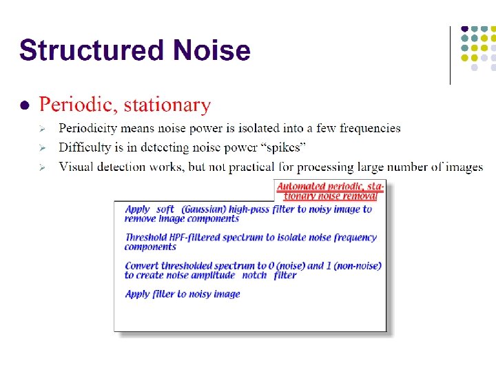
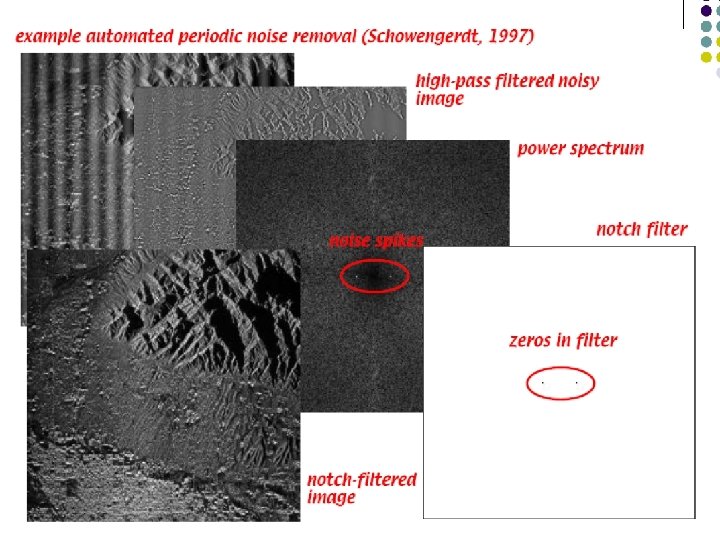
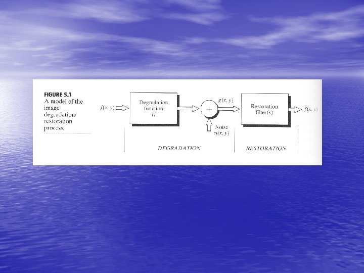
5 1 Model of Image degradation and restoration
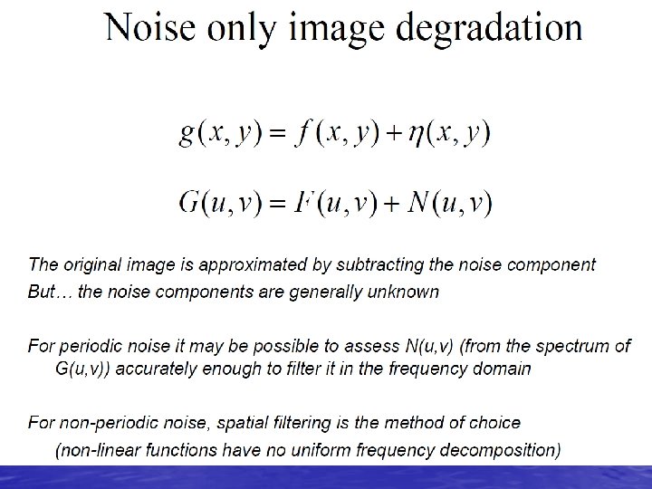
=h(x, y) f(x, y)+")

 • Gaussian noise – – – : mean; :")

 • Rayleigh noise • = a+( b/4)1/2 • =")
 • Erlang (gamma) noise • =b/a; =b/a 2")
 • Exponential noise • =1/a; =1/a 2 • A")
 • Uniform noise • =(a+b)/2; =(b-a)2/12")
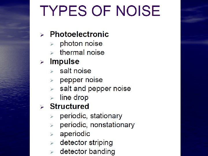
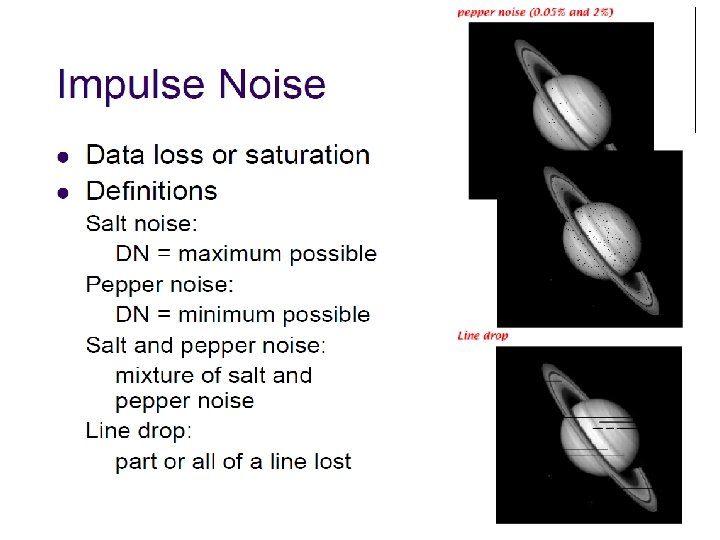
 • Impulse noise (salt and pepper noise)")


 • The recently proposed Nonlocal Means Algorithm (NLmeans) has")
 • Same goals: ‘Smooth within Similar Regions’ •")
 • For each and every pixel p:")
 • For each and every pixel p: – Define a")
 Vp = 0. 74 0. 32 0. 41 0. 55")
 q ‘Similar’ pixels p, q SMALL vector distance; || Vp")
 q ‘Dissimilar’ pixels p, q LARGE vector distance; || Vp")
 ‘Dissimilar’ pixels p, q LARGE vector distance; || Vp –")
 p, q neighbors define a vector distance; || Vp –")
 pixels p, q neighbors Set a vector distance; || Vp")
 • Noisy source image:")
 • Gaussian Filter Low noise, Low detail")
 • Anisotropic Diffusion (Note ‘stairsteps’: ~ piecewise constant)")
 • Bilateral Filter (better, but similar ‘stairsteps’:")
 • NL-Means: Sharp, Low noise, Few artifacts.")


 Original image corrupted by salt and pepper noise (p=5 %")
 If we smooth the image with a larger median filter, e. g. 7")
 Salt and pepper noise (20 %) Smoothed by")
 Salt and pepper noise (20 %) Median filtered")


, find f(x, y).")


- Slides: 81
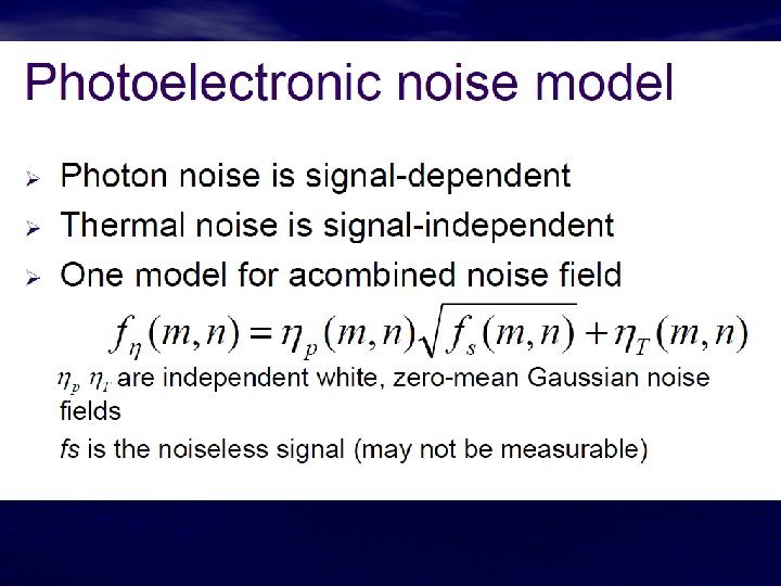
5. 1 Model of Image degradation and restoration • g(x, y)=h(x, y) f(x, y)+ (x, y) Note: H is a linear, position-invariant process.
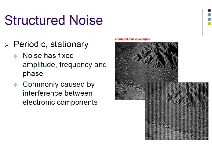
5. 2 Noise Model • Spatial and frequency property of noise – White noise (random noise) • A sequence of random positive/negative numbers whose mean is zero. – Independent of spatial coordinates and the image itself. • In the frequency domain, all the frequencies are the same. – All the frequencies are corrupted by an additional constant frequency. – Periodic noise
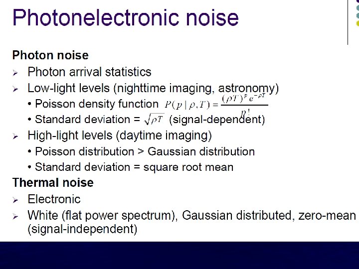
Noise Probability Density Functions (1) • Gaussian noise – – – : mean; : variance 70% [( - ), ( + )] 95 % [( -2 ), ( +2 )] • Because of its tractability, Gaussian (normal) noise model is often applicable at best.
Implementation • The problem of adding noise to an image is identical to that of adding a random number to the gray level of each pixel. – Noise models describe the distribution (probability density function, PDF) of these random numbers. – How to match the PDF of a group of random numbers to a specific noise model? • Histogram matching.
Noise Probability Density Functions (2) • Rayleigh noise • = a+( b/4)1/2 • = b(4 - )/4
Noise Probability Density Functions (3) • Erlang (gamma) noise • =b/a; =b/a 2
Noise Probability Density Functions (4) • Exponential noise • =1/a; =1/a 2 • A special case Erlang noise model when b = 1.
Noise Probability Density Functions (5) • Uniform noise • =(a+b)/2; =(b-a)2/12
Noise Probability Density Functions (6) • Impulse noise (salt and pepper noise)
Example
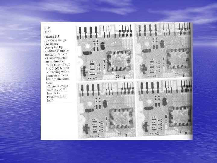
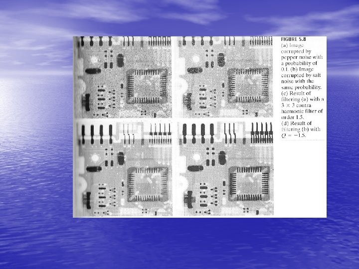
Results of adding noise
Results of adding noise
The Principle Use of Noise Models • Gaussian noise: • • – electronic circuit noise and sensor noise due to poor illumination or high temperature. Rayleigh noise: – Noise in range imaging. Erlang noise: – Noise in laser imaging. Impulse noise: – Quick transients take place during imaging. Uniform noise: – Used in simulations.
Impulse noise is caused by • Malfunctioning pixels in camera sensors • Fault memory locations in hardware • Transmisison in a noisy channel Two types: • Salt-and-pepper Noise • Uniformly-Distrubuted Random Noise
5. 2. 4 Estimation of Noise Parameters • How do we know which noise model adaptive to the currently available imaging tool? – Image a solid gray board that is illuminated uniformly. – Crop a small patch of constant grey level and analyze its histogram to see which model matches.
5. 2. 4 Estimation of Noise Parameters • Gaussian n: – Find the mean and standard deviation of the histogram (Gaussian noise). • Rayleigh, Erlang, and uniform noise: – Calculate the a and b from and . • Impulse noise: – Compute the height of peaks at gray levels 0 and 255 to find Pa and Pb.
Estimation of Noise Parameters
Non-Local Means Algorithm (Buades 2005) • The recently proposed Nonlocal Means Algorithm (NLmeans) has offered remarkably promising results. • Unlike previous denoising methods that rely on the local regularity assumption, the NL-means exploits spatial correlation in the entire image for noise removal. • It adjusts each pixel value with a weighted average of other pixels whose neighborhood has a similar geometrical configuration. • Since image pixels are highly correlated while noise is typically independently and identically distributed (i. i. d. ), averaging of these pixels results in noise cancellation and yields a pixel that is similar to its original value.
New Idea: NL-Means Filter (Buades 2005) • Same goals: ‘Smooth within Similar Regions’ • KEY INSIGHT: Generalize, extend ‘Similarity’ – Bilateral: Averages neighbors with similar intensities;
NL-Means Method: Buades (2005) • For each and every pixel p:
NL-Means Method: Buades (2005) • For each and every pixel p: – Define a small, simple fixed size neighborhood;
NL-Means Method: Buades (2005) Vp = 0. 74 0. 32 0. 41 0. 55 … … … • For each and every pixel p: – Define a small, simple fixed size neighborhood; – Define vector Vp: a list of neighboring pixel values.
NL-Means Method: Buades (2005) q ‘Similar’ pixels p, q SMALL vector distance; || Vp – Vq ||2 p
NL-Means Method: Buades (2005) q ‘Dissimilar’ pixels p, q LARGE vector distance; || Vp – Vq ||2 p q
NL-Means Method: Buades (2005) ‘Dissimilar’ pixels p, q LARGE vector distance; || Vp – Vq ||2 Filter with this! p q
NL-Means Method: Buades (2005) p, q neighbors define a vector distance; || Vp – Vq ||2 Filter with this: No spatial term! p q
NL-Means Method: Buades (2005) pixels p, q neighbors Set a vector distance; || Vp – Vq ||2 Vector Distance to p sets weight for each pixel q p q
NL-Means Filter (Buades 2005) • Noisy source image:
NL-Means Filter (Buades 2005) • Gaussian Filter Low noise, Low detail
NL-Means Filter (Buades 2005) • Anisotropic Diffusion (Note ‘stairsteps’: ~ piecewise constant)
NL-Means Filter (Buades 2005) • Bilateral Filter (better, but similar ‘stairsteps’:
NL-Means Filter (Buades 2005) • NL-Means: Sharp, Low noise, Few artifacts.
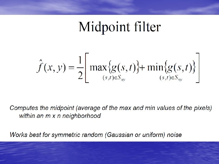
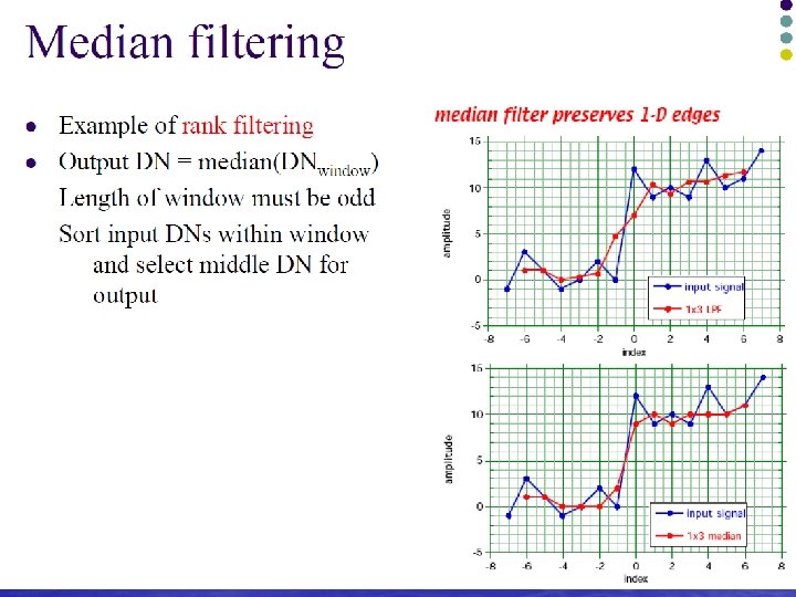
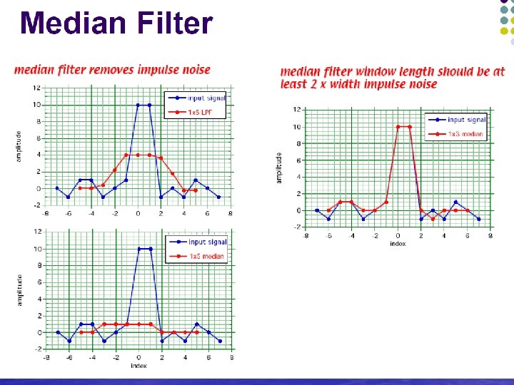
Order-Statistics filters • Median filter • Max filter: find the brightest points to reduce the pepper noise • Min filter: find the darkest point to reduce the salt noise • Midpoint filter: combining statistics and averaging.
Median filter
The median filter is used for removing noise. It can remove isolated impulsive noise and at the same time it preserves the edges and other structures in the image. Contrary to average filtering it does not smooth the edges.
Unlike the mean filter, the median filter is non -linear. This means that for two images A(x) and B(x):
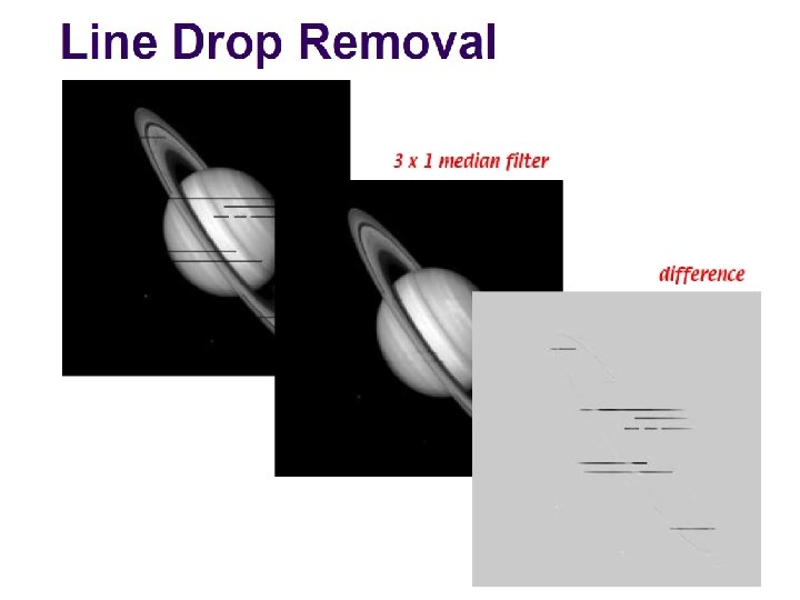
Removal of Line Artifacts by Median Filtering
The original image. b) Original image corrupted by salt and pepper noise (p=5 % that a bit is flipped. c) After smoothing with a 3 x 3 filter most of the noise has been eliminated.
d) If we smooth the image with a larger median filter, e. g. 7 x 7, all the noise pixels disappear. e) Alternatively, we can pass a 3 x 3 filter over the image 3 times in order to remove the noise with less loss of detail.
Salt and pepper noise (5 %) Salt and pepper noise (20 %) Smoothed by 3 x 3 window
Salt and pepper noise (5 %) Salt and pepper noise (20 %) Median filtered by 3 x 3 window
Example 5. 3 Iteratively applying median filter to an image corrupted by impulse noise.
Alpha-trimmed mean filter is windowed filter of nonlinear class, by its nature is hybrid of the mean and median filters. The basic idea behind filter is for any element of the signal (image) look at its neighborhood, discard the most atypical elements and calculate mean value using the rest of them.
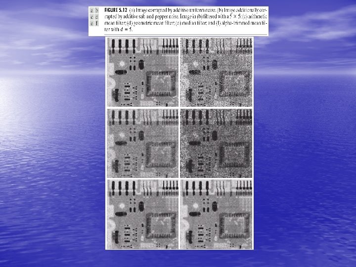
Alpha-Trimmed Mean Filter • Combining the advantages of mean filter and order-statistics filter. – Suppose delete d/2 lowest and d/2 highest gray-level value in the neighborhood of Sxy and average the remaining mn-d pixel, denoted by gr(s, t). where d=0 ~ mn-1
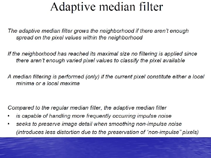
Adaptive Filter • Filters whose behavior changes based • on statistical characteristics of the image. Two adaptive filters are considered: (1) Adaptive, local noise reduction filter. (2) Adaptive median filter.
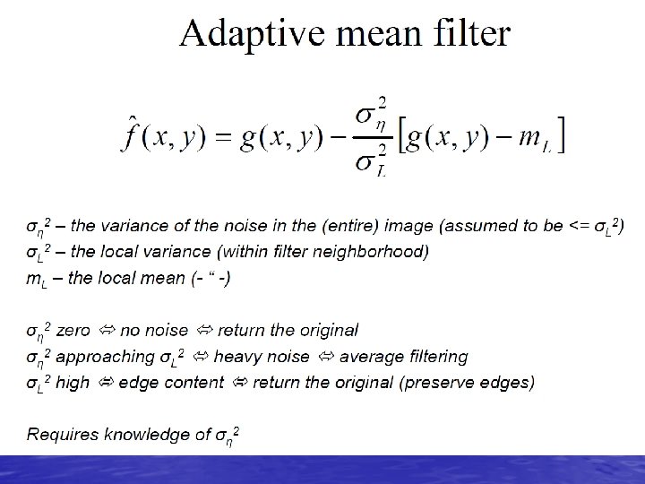
Adaptive, Local Noise Reduction Filter • Two parameters are considered: – Mean: measure of average gray level. – Variance: measure of average contrast. • Four measurements: (1) noisy image at (x, y ): g(x, y ) (2) The variance of noise 2 (3) The local mean m. L in Sxy (4) The local variance 2 L
Adaptive, Local Noise Reduction Filter Given the corrupted image g(x, y), find f(x, y). Conditions: (a) 2 is zero (Zero-noise case) – Simply return the value of g(x, y). (b) If 2 L is higher than 2 – Could be edge and should be preserved. – Return value close to g(x, y). (c) If 2 L = 2 – when the local area has similar properties with the overall image. – Return arithmetic mean value of the pixels in Sxy. General expression:
Adaptive, Local Noise Reduction Filter
Adaptive Median Filter • Adaptive median filter can handle impulse • • noise with larger probability (Pa and Pb are large). This approach changes window size during operation (according to certain criteria). First, define the following notations: zmin=minimum gray-level value in Sxy zmax=maximum gray-level value in Sxy zmed=median gray-level value in Sxy zxy= gray-level at (x, y) Smax=maximum allowed size of Sxy
Adaptive Median Filter • The adaptive median filter algorithm works • in two levels: A and B Level A: A 1=zmed-zmin A 2=zmed-zmax If A 1>0 and A 2<0 goto level B else increase the window size If window size Smax repeat level A else output zxy Level B: B 1=zxy-zmin B 2=zxy-zmax If B 1>0 AND B 2<0, output zxy Else output zmed.
Example 5. 5
Salt and pepper noise Salt and Pepper Standard Median output Adaptive median Output
With Non-impulsive noise Gaussian Noise Standard Median output Adaptive Median Output
With both types of noise Gaussian and impulsive Noise Standard Median output Adaptive Median output
Conclusions • The adaptive median filter successfully removes • • impulsive noise from images. It does a reasonably good job of smoothening images that contain non -impulsive noise. When both types of noise are present, the algorithm is not as successful in removing impulsive noise and its performance deteriorates. Overall, the performance is as expected and the successful implementation of the adaptive median filter is presented.
The End