2 nd Annual French Complex Systems Summer School

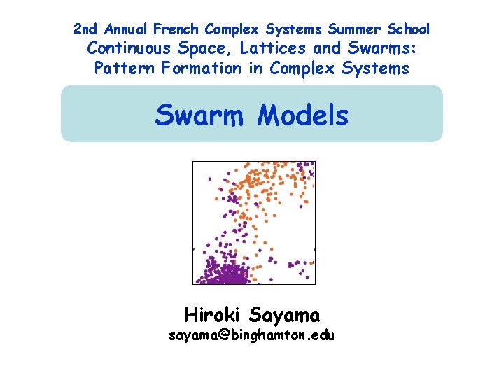
2 nd Annual French Complex Systems Summer School Continuous Space, Lattices and Swarms: Pattern Formation in Complex Systems Swarm Models Hiroki Sayama sayama@binghamton. edu

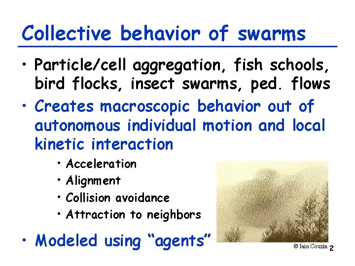
Collective behavior of swarms • Particle/cell aggregation, fish schools, bird flocks, insect swarms, ped. flows • Creates macroscopic behavior out of autonomous individual motion and local kinetic interaction • • Acceleration Alignment Collision avoidance Attraction to neighbors • Modeled using “agents” © Iain Couzin 2

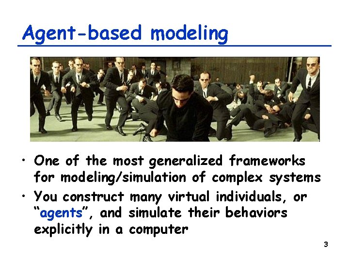
Agent-based modeling • One of the most generalized frameworks for modeling/simulation of complex systems • You construct many virtual individuals, or “agents”, and simulate their behaviors explicitly in a computer 3

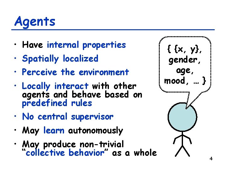
Agents • Have internal properties • Spatially localized • Perceive the environment • Locally interact with other agents and behave based on predefined rules { {x, y}, gender, age, mood, … } • No central supervisor • May learn autonomously • May produce non-trivial “collective behavior” as a whole 4

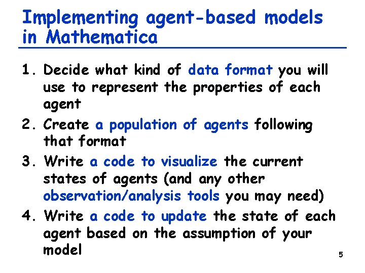
Implementing agent-based models in Mathematica 1. Decide what kind of data format you will use to represent the properties of each agent 2. Create a population of agents following that format 3. Write a code to visualize the current states of agents (and any other observation/analysis tools you may need) 4. Write a code to update the state of each agent based on the assumption of your model 5

Models with Fixed Number of Agents 6

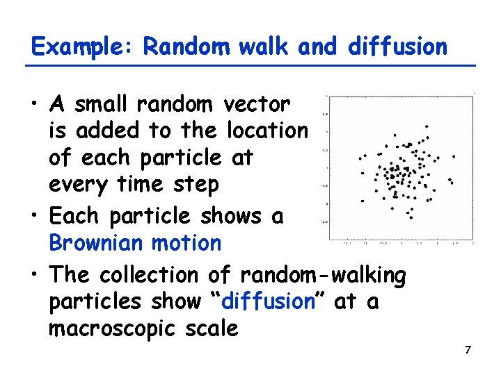
Example: Random walk and diffusion • A small random vector is added to the location of each particle at every time step • Each particle shows a Brownian motion • The collection of random-walking particles show “diffusion” at a macroscopic scale 7

Exercise • Modify the “random walk” simulator code so that: – Each particle has its own velocity – Each particle is accelerated by the attractive force toward the “center of mass” of the population of particles This should create a simple swarming behavior 8

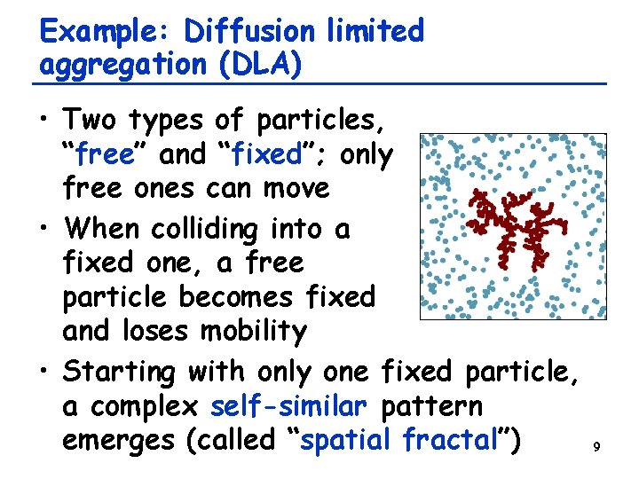
Example: Diffusion limited aggregation (DLA) • Two types of particles, “free” and “fixed”; only free ones can move • When colliding into a fixed one, a free particle becomes fixed and loses mobility • Starting with only one fixed particle, a complex self-similar pattern emerges (called “spatial fractal”) 9

Exercise • Carry out the DLA simulation runs with multiple “seeds” randomly positioned in the space • Modify the simulator code so that (1) initially no “fixed” particles exist, but (2) the particles that touched the bottom edge of the space turn to “fixed” 10

Models with Agent-Environment Interaction 11

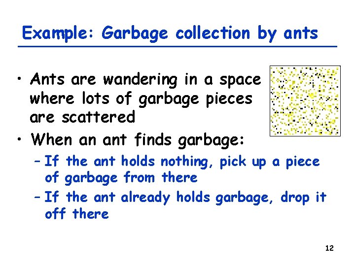
Example: Garbage collection by ants • Ants are wandering in a space where lots of garbage pieces are scattered • When an ant finds garbage: – If the ant holds nothing, pick up a piece of garbage from there – If the ant already holds garbage, drop it off there 12

Exercise • Modify the ants’ garbage collection model so that: – Each ant produces pheromone where it is – Pheromone diffuses and evaporates at a constant rate – Ants are stochastically attracted toward places where there are greater amount of pheromone 13

Models with Agent Replacement 14

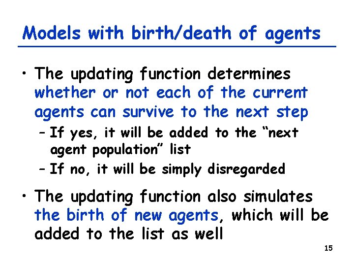
Models with birth/death of agents • The updating function determines whether or not each of the current agents can survive to the next step – If yes, it will be added to the “next agent population” list – If no, it will be simply disregarded • The updating function also simulates the birth of new agents, which will be added to the list as well 15

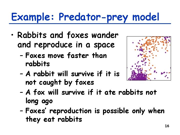
Example: Predator-prey model • Rabbits and foxes wander and reproduce in a space – Foxes move faster than rabbits – A rabbit will survive if it is not caught by foxes – A fox will survive if it ate rabbits not long ago – Foxes’ reproduction is possible only when they eat rabbits 16

Exercise • Modify the simulator code so that it outputs the time series plots of rabbit and fox populations in addition to the visual image of simulation • See if you actually have oscillatory behavior in these plots 17

Exercise: Evolutionary adaptation • Make the range of motion (motility) a heritable individual property of agents • Introduce mutations of the agent motility in both foxes and rabbits • See how the agent motilities spontaneously evolve in simulation 18

Exercise: Evolutionary adaptation • Make the reproduction of agent density-dependent – Too few neighbors / too many neighbors will result in failure of reproduction • See how the agent motilities spontaneously evolve in simulation 19

Pattern Formation in Heterogeneous Particle Swarms: “Swarm Chemistry” 20

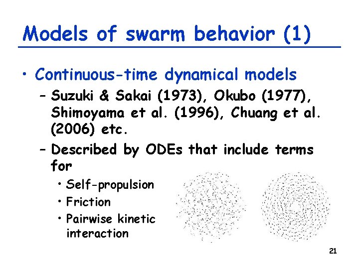
Models of swarm behavior (1) • Continuous-time dynamical models – Suzuki & Sakai (1973), Okubo (1977), Shimoyama et al. (1996), Chuang et al. (2006) etc. – Described by ODEs that include terms for • Self-propulsion • Friction • Pairwise kinetic interaction 21

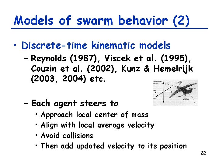
Models of swarm behavior (2) • Discrete-time kinematic models – Reynolds (1987), Viscek et al. (1995), Couzin et al. (2002), Kunz & Hemelrijk (2003, 2004) etc. – Each agent steers to • • Approach local center of mass Align with local average velocity Avoid collisions Then add updated velocity to its position 22

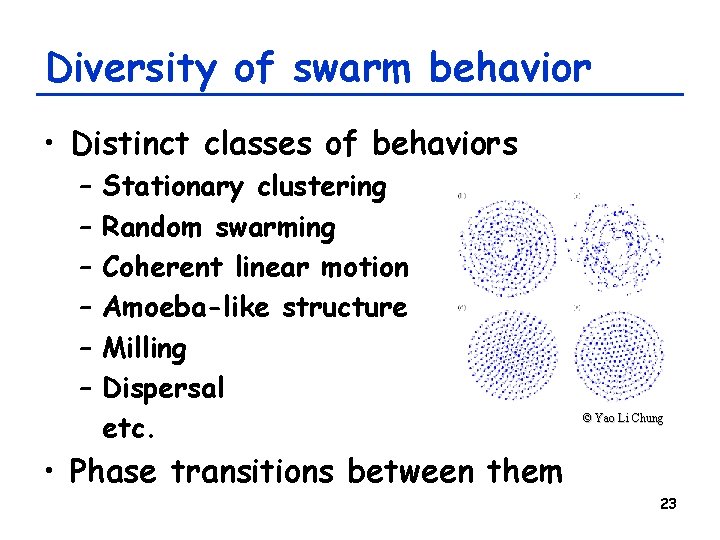
Diversity of swarm behavior • Distinct classes of behaviors – – – Stationary clustering Random swarming Coherent linear motion Amoeba-like structure Milling Dispersal etc. © Yao Li Chung • Phase transitions between them 23

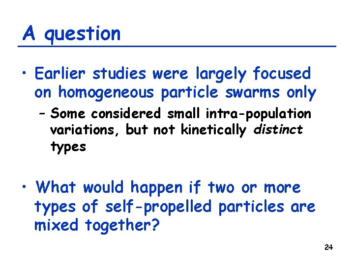
A question • Earlier studies were largely focused on homogeneous particle swarms only – Some considered small intra-population variations, but not kinetically distinct types • What would happen if two or more types of self-propelled particles are mixed together? 24

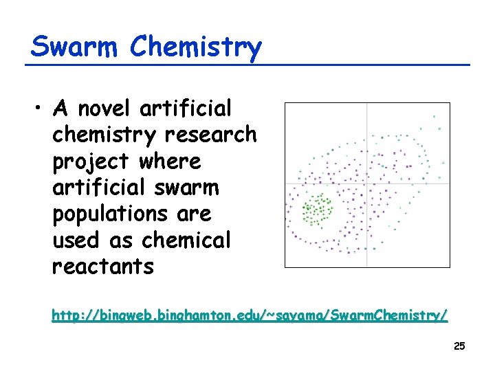
Swarm Chemistry • A novel artificial chemistry research project where artificial swarm populations are used as chemical reactants http: //bingweb. binghamton. edu/~sayama/Swarm. Chemistry/ 25

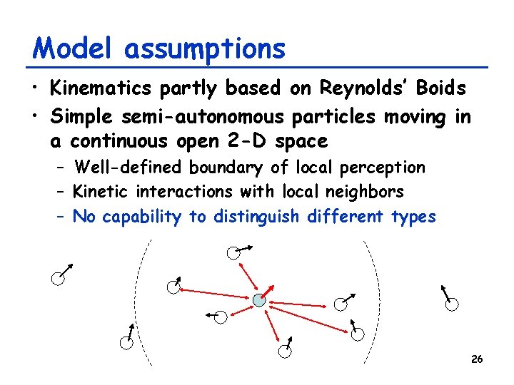
Model assumptions • Kinematics partly based on Reynolds’ Boids • Simple semi-autonomous particles moving in a continuous open 2 -D space – Well-defined boundary of local perception – Kinetic interactions with local neighbors – No capability to distinguish different types 26

Behavioral rules • If no particles are found within local perception range, steer randomly (Straying) • Otherwise: – Steer to move toward the average position of local neighbors (Cohesion) – Steer towards the average velocity of local neighbors (Alignment) – Steer to avoid collision with neighbors (Separation) – Steer randomly with a given probability (Randomness) • Approximate its speed to its normal speed (Self-propulsion) 27

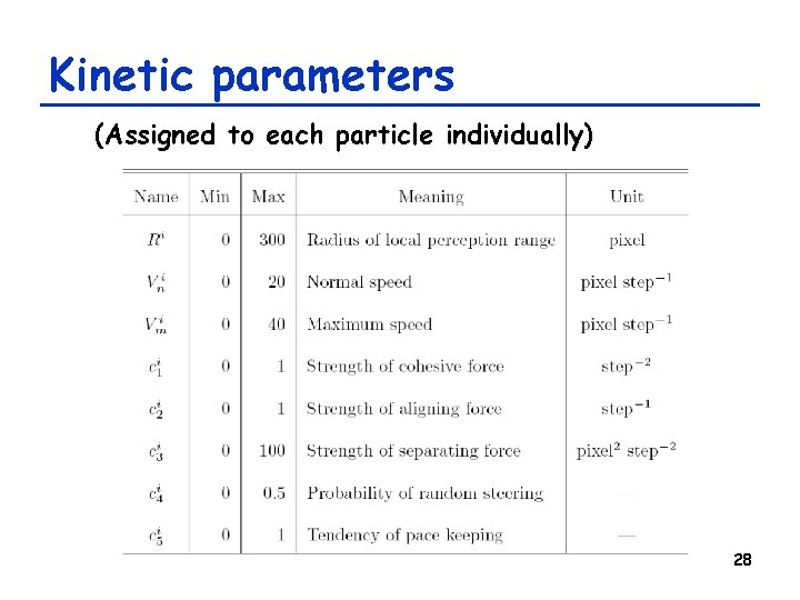
Kinetic parameters (Assigned to each particle individually) 28

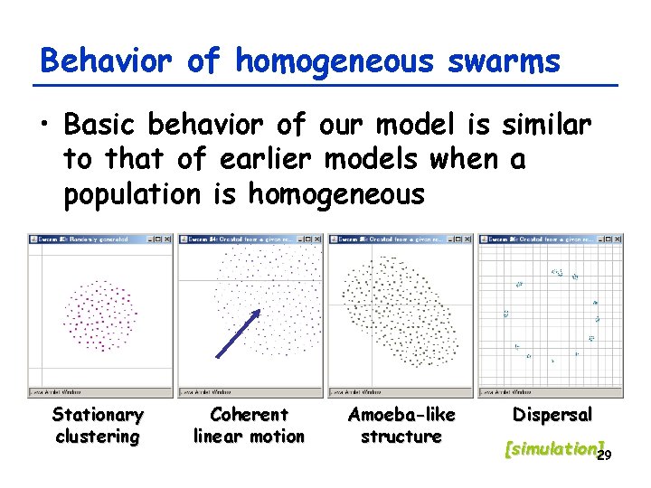
Behavior of homogeneous swarms • Basic behavior of our model is similar to that of earlier models when a population is homogeneous Stationary clustering Coherent linear motion Amoeba-like structure Dispersal [simulation]29

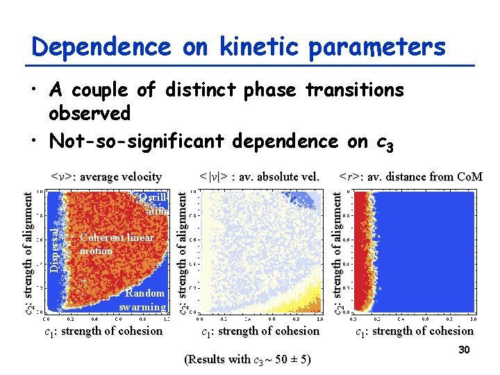
Dependence on kinetic parameters • A couple of distinct phase transitions observed • Not-so-significant dependence on c 3 Random swarming c 1: strength of cohesion <r>: av. distance from Co. M c 2: strength of alignment Coherent linear motion <|v|> : av. absolute vel. c 2: strength of alignment Oscillation Dispersal c 2: strength of alignment <v>: average velocity c 1: strength of cohesion (Results with c 3 ~ 50 ± 5) c 1: strength of cohesion 30

[simulation] Exploring pairwise interactions • Monte Carlo simulations (> 50, 000 runs) • Fixed parameters: – N=300, R=200, Vn=10, Vm=40, c 4=0, c 5=0. 5 • Varied parameters: – c 1, c 2, c 3 (cohesion, alignment, separation) – Two types (A, B) of particles randomly created; simulate each in isolation as well as in mixture • Initial conditions: – Randomly positioned and oriented in a 300 x 300 space • Quantities measured after 200 time steps: – Average linear/angular velocities, average distance from center of mass, local homogeneity 31

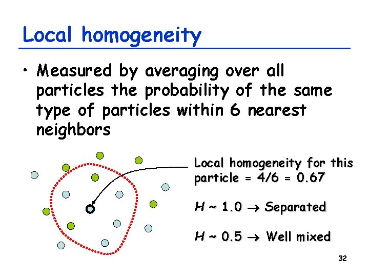
Local homogeneity • Measured by averaging over all particles the probability of the same type of particles within 6 nearest neighbors Local homogeneity for this particle = 4/6 = 0. 67 H ~ 1. 0 Separated H ~ 0. 5 Well mixed 32

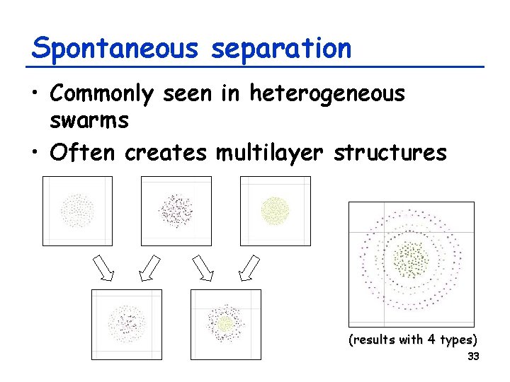
Spontaneous separation • Commonly seen in heterogeneous swarms • Often creates multilayer structures (results with 4 types) 33

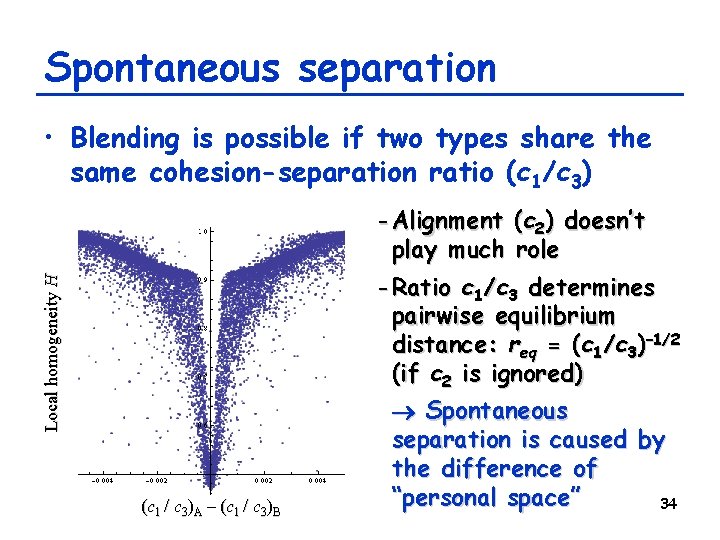
Spontaneous separation Local homogeneity H • Blending is possible if two types share the same cohesion-separation ratio (c 1/c 3) (c 1 / c 3 )A – (c 1 / c 3 )B - Alignment (c 2) doesn’t play much role - Ratio c 1/c 3 determines pairwise equilibrium distance: req = (c 1/c 3)– 1/2 (if c 2 is ignored) Spontaneous separation is caused by the difference of “personal space” 34

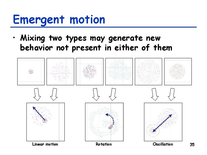
Emergent motion • Mixing two types may generate new behavior not present in either of them Linear motion Rotation Oscillation 35

Interactions between >2 types? • Possibility space explodes exponentially with # of types involved – Exhaustive parameter sweep not feasible – Monte Carlo may not give enough resolution • It is no longer clear what kind of quantities should be measured to characterize resulting patterns – We don’t know what to expect 36

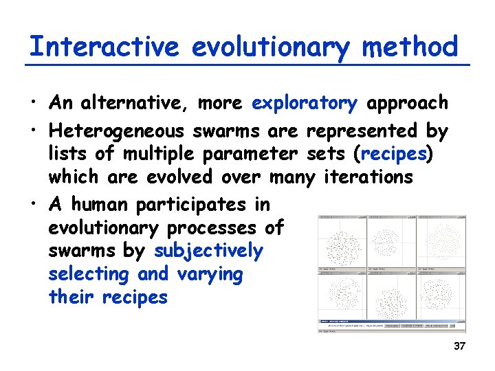
Interactive evolutionary method • An alternative, more exploratory approach • Heterogeneous swarms are represented by lists of multiple parameter sets (recipes) which are evolved over many iterations • A human participates in evolutionary processes of swarms by subjectively selecting and varying their recipes 37

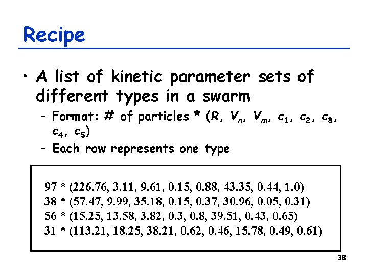
Recipe • A list of kinetic parameter sets of different types in a swarm – Format: # of particles * (R, Vn, Vm, c 1, c 2, c 3, c 4, c 5) – Each row represents one type 97 * (226. 76, 3. 11, 9. 61, 0. 15, 0. 88, 43. 35, 0. 44, 1. 0) 38 * (57. 47, 9. 99, 35. 18, 0. 15, 0. 37, 30. 96, 0. 05, 0. 31) 56 * (15. 25, 13. 58, 3. 82, 0. 3, 0. 8, 39. 51, 0. 43, 0. 65) 31 * (113. 21, 18. 25, 38. 21, 0. 62, 0. 46, 15. 78, 0. 49, 0. 61) 38

[simulation] 39

Evolutionary operators (1) • Perturbation to relative frequencies of different parameter sets within a recipe • Mixing of two swarms physically 40

Evolutionary operators (2) • Duplication of parameter sets • Deletion of parameter sets • Insertion of new parameter sets • Point mutation of parameter values 41

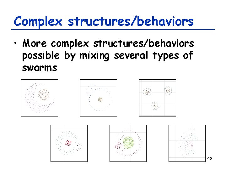
Complex structures/behaviors • More complex structures/behaviors possible by mixing several types of swarms 42

Summary • Many physical/biological/ecological systems can be modeled as swarms using agent-based modeling – Can include local interaction, heterogeneity, interaction with environment, birth/death of agents, etc. • Heterogeneous swarms may selforganize and robustly produce complex patterns (structures and behaviors) 43