Summer School 2013 Economics of Food Safety Competitiveness























- Slides: 47

Summer School 2013 Economics of Food Safety, Competitiveness and Applied Microeconometrics Hedonic pricing method Revealed preferences No questionnaire! We gather data that come from the market No need to build a hypothetical market Where do we decide to live? Why do we choose a specific location? Which factors push companies to choose one location rather than another? Which characteristics of an area affect housing prices? Which are the important elements of a house that determine its price? 1

Summer School 2013 Economics of Food Safety, Competitiveness and Applied Microeconometrics The choice of localization The choice of housing is a composite good Distance from work, availability of public services, distance from schools, availability of green areas, availability of sport facilities, characteristics of housing (# of bedrooms, # of bathrooms, flat, detached, etc. ) etc. We assume that buyers choose houses that maximize their utility The constraints in the maximization problem are given by income, the price of the houses and the level of taxes => therefore, the housing market give us some information on buyers preferences for housing and for their localization 2

Summer School 2013 Economics of Food Safety, Competitiveness and Applied Microeconometrics Composite goods Goods (or sites) can be described by a set of attributes or characteristics. The hedonic pricing method uses the same idea that goods are composed by a set of characteristics. Consider the characteristics of a house: Number of floors, presence of a garden, number of bedrooms, number of bathrooms, square footage of the house, type of house, age, materials, etc. And also: Distance from public transport, distance from the city centre, distance from main roads, distance from shops, distance from sport facilities, crime rate, average income of inhabitants, presence of a university, etc. The composite good has a price, but there is no explicit price for each characteristic that compose the good. 3

Summer School 2013 Economics of Food Safety, Competitiveness and Applied Microeconometrics The hedonic pricing method Problem of estimating hedonic equations Hedonic prices are identified through a comparison of similar goods that differ for the quality of one characteristic The basic idea is to use the systematic variation in the price of a good that can be explained by an environmental characteristic of the good. This is the starting point to assess the WTP for the environmental characteristic We look at market data! Real transactions! 4

Summer School 2013 Economics of Food Safety, Competitiveness and Applied Microeconometrics Example Let’s consider 2 residential properties identical in all characteristics and localization. The only difference is that house A has 2 bedrooms, while house B has 3 bedrooms. In a competitive market, the price difference between the two houses reflects the value of the additional room of house B. If the price difference between the two houses is less than buyers’ WTP for the additional room, then buyers will try to buy house B, driving up its price until the equilibrium is reached. In the same way, if house A costs much less than house B, buyers will increase the demand for house A, driving up its price. 5

Summer School 2013 Economics of Food Safety, Competitiveness and Applied Microeconometrics The hedonic pricing method applies this simple concept to the environmental characteristics of residential properties The price difference between houses that have different levels of environmental quality, keeping constant all other characteristics, reflects the WTP for the different level of environmental quality => we can assess the value of an environmental quality, according to market prices of residential properties => variation in environmental quality affects the price of housing 6

Summer School 2013 Economics of Food Safety, Competitiveness and Applied Microeconometrics A bit of history 1926 Waugh studies the variation of prices of vegetables 1938 Court looks at the car market in Detroit 1967 first application to the housing market: Ridker and Henning => effects of air pollution on prices of housing 1974 Rosen describe the first formal model of the hedonic pricing method Other applications: ◦ ◦ Agricultural goods Cars Wine Job market 7

Summer School 2013 Economics of Food Safety, Competitiveness and Applied Microeconometrics Rosen’s model Consumers (buyers) have a utility function: U(s, n, c) s = house characteristics n = characteristics of the area where the house is located c = other consumption goods Budget constraint: m = c + p(s, n) m = income p(s, n) expenditure for a house p(s, n) is assumed to change in a non linear relationship with the characteristics of houses. That is, the cost of houses change in an unknown relationship with number of rooms, etc. c is the expenditure for all other goods 8

Summer School 2013 Economics of Food Safety, Competitiveness and Applied Microeconometrics The maximization of the utility function subject to the budget constraint, gives the usual first order conditions. That is, the marginal rate of substitution between each characteristic n and the consumption of other goods is equal to the ‘price’ (coefficient) of n and the price of c. The price of c is our numeraire and we put it equal to 1. The price of n describes the price of a marginal change in n. The first order conditions are: (Un is the partial derivative of U with respect to n) First order conditions simply say that the consumer (buyer) is willing to pay pn for a marginal change of n 9

Summer School 2013 Economics of Food Safety, Competitiveness and Applied Microeconometrics Utility maximization and budget constraint c U(s*, n, c) m=c+p(s*, n) n 10

Summer School 2013 Economics of Food Safety, Competitiveness and Applied Microeconometrics The hedonic price function The function that describes how housing price changes when housing characteristics change: p(s, n) is the hedonic price function The derivative of the function with respect to one of the characteristics n is the ‘implicit price’ of n. If we knew the hedonic price function and the implicit price of n, we could estimate buyers’ WTP for n, given that this is equal to the marginal rate of substitution between n and the other goods (numeraire) 11

Summer School 2013 Economics of Food Safety, Competitiveness and Applied Microeconometrics Indifference curves The budget constraint says that we don’t spend for other goods is spent for housing: p(s, n): c = m – p(s, n) The utility function can be written in this way: U(s, n, c)=U(s, n, m – p(s, n)) Therefore we can describe the utility function of consumers (buyers) with indifference curves (for given values of m and s): Each indifference curve gives for a constant level of utility the expenditure on housing and n for a given level of income and s. p(s*. n) U n 12

Summer School 2013 Economics of Food Safety, Competitiveness and Applied Microeconometrics Heterogeneous consumers People with different incomes have different indifference curves, even if they have the same preferences (U has the same functional form for all respondents) People with different preferences have different indifference curves In a world of heterogeneous consumers (buyers) that have different levels of income, we have a continuum of indifference curves: p(s*. n) n 13

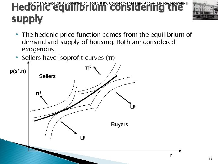
Summer School 2013 Economics of Food Safety, Competitiveness and Applied Microeconometrics Hedonic equilibrium Suppose that consumers (buyers) consider exogenous the hedonic price function Consumers (buyers) maximize utility subject to the budget constraint and to the hedonic price function: p(s*. n) n 14

Hedonic equilibrium considering the supply Summer School 2013 Economics of Food Safety, Competitiveness and Applied Microeconometrics The hedonic price function comes from the equilibrium of demand supply of housing. Both are considered exogenous. Sellers have isoprofit curves (π) p(s*. n) πb Sellers πa Uk Buyers Ui n 15

Summer School 2013 Economics of Food Safety, Competitiveness and Applied Microeconometrics Marginal Willingness To Pay The main characteristic of the model is that buyers and sellers are efficiently matched along the hedonic price function At any point along the hedonic price function, buyers marginal willingness to pay (and sellers willingness to accept) for a change in n is given by the derivative of the hedonic price function with respect to n. This implicit price changes with n if the hedonic price function is non linear. The model can be generalized to the case where we consider several characteristics of residential properties and of the area where houses are located: p(x 1, x 2, …xk) 16

Summer School 2013 Economics of Food Safety, Competitiveness and Applied Microeconometrics Model estimate Now we need to specify a functional form for p. A common functional form is the double-log: The implicit price can be estimated for specific value of the characteristics of houses (for example, the average value) For the double-log function, the implicit price of x 1 is given by: β 1 gives the percentage change in the price of housing given a percentage change in x 1 We usually estimate the implicit price at the average value of housing 17

Summer School 2013 Economics of Food Safety, Competitiveness and Applied Microeconometrics Some limitations and assumptions Perfect information: Buyers can purchase whatever combination of characteristics they desire. ◦ Buyers observe the characteristics of houses and are able to perfectly describe the hedonic price function ◦ They can always find the combination of bedrooms, bathrooms, location of the house that they want Implicit prices allow us only to assess marginal variations in the characteristics of houses (but if we consider that all buyers are identical then we can consider non marginal changes as well – too strong assumption!) ◦ Example: if the average house has 3 bedrooms and costs X, I cannot say that buyers are willing to pay Y for a house that has 7 bedrooms. We can’t say that an increase of 4 bedrooms is a marginal change The estimate of non-marginal variations requires the estimate of individual demand parameters, which is very difficult 18

Summer School 2013 Economics of Food Safety, Competitiveness and Applied Microeconometrics Econometric problems Multicollinearity Heteroskedasticity Spatial autocorrelation ◦ if a house has several bedrooms, it will likely have several bathrooms, etc. ◦ distances: don’t use too many distances in your function ◦ The value of one house will be influenced by the value of surrounding houses If I only use the data of sold properties and do not consider the characteristics of unsold properties, my coefficient can be biased (sample selection bias) ◦ Solution: 2 steps estimate 1) Probit model for the probability of a sale with both sold and unsold properties 2) regression model with only sold properties + Inverse Mills Ratio calculated in 1. Check if the coefficient of the inverse mills ratio is significantly different from zero. If it is not, then delete it from the regression 19

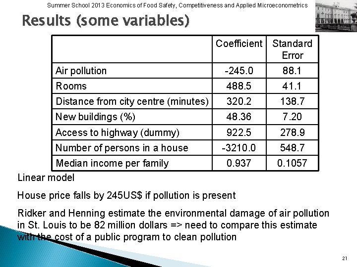
Summer School 2013 Economics of Food Safety, Competitiveness and Applied Microeconometrics Example 1: Air quality Air pollution is one of the first application of the hedonic pricing model Ridker, Henning (1967) “The determinants of property values with special reference to air pollution” Review of Economics and Statistics. No residential properties sale prices, but census tract data from St. Luis, 1960. Dependent variable: median value of property prices Independent variables: median characteristics of houses in a census tract, quality of schooling, access to highway, neighbourhood characteristics, tax levels, public services Air quality (SO 2, SO 3, H 2 SO 4) measured as direct effects on houses and on human health. 20

Summer School 2013 Economics of Food Safety, Competitiveness and Applied Microeconometrics Results (some variables) Coefficient Standard Error Air pollution -245. 0 88. 1 Rooms 488. 5 41. 1 Distance from city centre (minutes) 320. 2 138. 7 New buildings (%) 48. 36 7. 20 Access to highway (dummy) 922. 5 278. 9 -3210. 0 548. 7 0. 937 0. 1057 Number of persons in a house Median income per family Linear model House price falls by 245 US$ if pollution is present Ridker and Henning estimate the environmental damage of air pollution in St. Louis to be 82 million dollars => need to compare this estimate with the cost of a public program to clean pollution 21

Summer School 2013 Economics of Food Safety, Competitiveness and Applied Microeconometrics Problems of Ridker e Henning example Multicollinearity Omitted variables Positive sign for the coefficient of the distance from the city centre They do not consider the price of single houses, but the median value of the houses sold in a census tract … 22

Summer School 2013 Economics of Food Safety, Competitiveness and Applied Microeconometrics Example 2: Water quality Leggett and Bockstael (2000) Journal of Environmental Economics and Management 741 observations Effects of Chesapeake Bay water quality on prices of houses located along the bay Rather than using the characteristics of houses (rooms, bathrooms, etc. ), Leggett and Bockstael use the appraised value of houses. Water quality is measured using information on the level of pollution of the bay publicly given by the Department of Health of Maryland 23

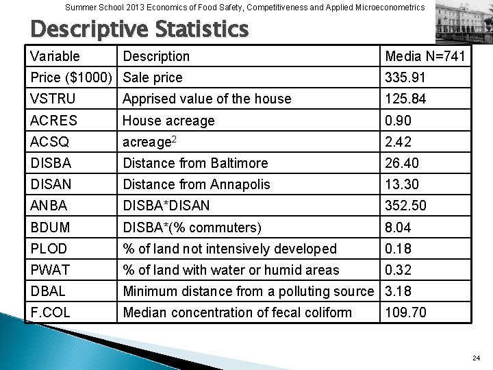
Summer School 2013 Economics of Food Safety, Competitiveness and Applied Microeconometrics Descriptive Statistics Variable Description Media N=741 Price ($1000) Sale price 335. 91 VSTRU Apprised value of the house 125. 84 ACRES House acreage 0. 90 ACSQ acreage 2 2. 42 DISBA Distance from Baltimore 26. 40 DISAN Distance from Annapolis 13. 30 ANBA DISBA*DISAN 352. 50 BDUM DISBA*(% commuters) 8. 04 PLOD % of land not intensively developed 0. 18 PWAT % of land with water or humid areas 0. 32 DBAL Minimum distance from a polluting source 3. 18 F. COL Median concentration of fecal coliform 109. 70 24

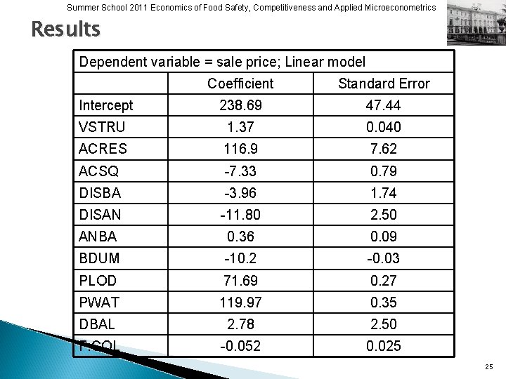
Summer School 2011 Economics of Food Safety, Competitiveness and Applied Microeconometrics Results Dependent variable = sale price; Linear model Coefficient Standard Error Intercept 238. 69 47. 44 VSTRU 1. 37 0. 040 ACRES 116. 9 7. 62 ACSQ -7. 33 0. 79 DISBA -3. 96 1. 74 DISAN -11. 80 2. 50 ANBA 0. 36 0. 09 BDUM -10. 2 -0. 03 PLOD 71. 69 0. 27 PWAT 119. 97 0. 35 DBAL 2. 78 2. 50 F. COL -0. 052 0. 025 25

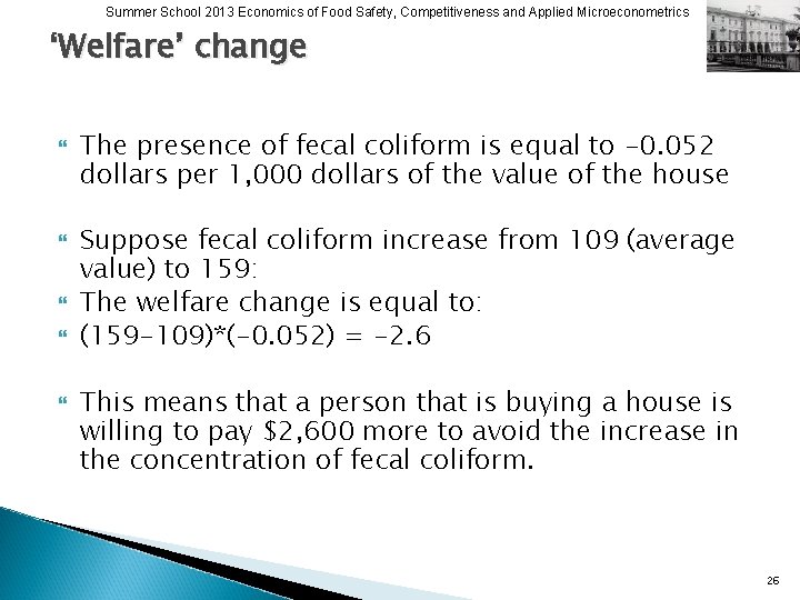
Summer School 2013 Economics of Food Safety, Competitiveness and Applied Microeconometrics ‘Welfare’ change The presence of fecal coliform is equal to -0. 052 dollars per 1, 000 dollars of the value of the house Suppose fecal coliform increase from 109 (average value) to 159: The welfare change is equal to: (159 -109)*(-0. 052) = -2. 6 This means that a person that is buying a house is willing to pay $2, 600 more to avoid the increase in the concentration of fecal coliform. 26

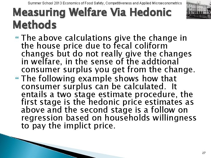
Summer School 2013 Economics of Food Safety, Competitiveness and Applied Microeconometrics Measuring Welfare Via Hedonic Methods The above calculations give the change in the house price due to fecal coliform changes but do not really give the changes in welfare, in the sense of the addtional consumer surplus you get from the change. The following example shows how that consumer surplus can be calculated. It entails a two stage estimate procedure, the first stage is the hedonic price estimates as above and the second stage is a follow on regression based on households willingness to pay the implict price. 27

Summer School 2013 Economics of Food Safety, Competitiveness and Applied Microeconometrics Case Study - Overview This exercise presents an application of the Hedonic Price Method for the valuation of benefits brought about by the improvement of the broadleaf coverage rate in an urban area. The local government decided to improve the quality of urban parks and green spaces near residential areas. F. Caracciolo Case Study N. 1, Portici 2011 28

Summer School 2013 Economics of Food Safety, Competitiveness and Applied Microeconometrics Case Study - Overview This study focuses on the valuation of only one of them, namely the increase of broadleaf coverage. To elicit the value assigned to a change in broadleaf coverage, the prices of houses in areas with different coverage rates are observed. F. Caracciolo Case Study N. 1, Portici 2011 29

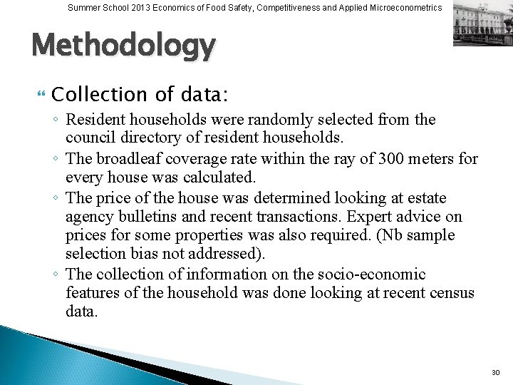
Summer School 2013 Economics of Food Safety, Competitiveness and Applied Microeconometrics Methodology Collection of data: ◦ Resident households were randomly selected from the council directory of resident households. ◦ The broadleaf coverage rate within the ray of 300 meters for every house was calculated. ◦ The price of the house was determined looking at estate agency bulletins and recent transactions. Expert advice on prices for some properties was also required. (Nb sample selection bias not addressed). ◦ The collection of information on the socio-economic features of the household was done looking at recent census data. 30

Summer School 2013 Economics of Food Safety, Competitiveness and Applied Microeconometrics Methodology Calculation of the value of environmental quality: ◦ Estimation of the House Price Function. ◦ Calculation of the Implicit Marginal Price of the environmental good (the responsiveness of the house price function with respect to the environmental quality, ie the first derivative: c x P/Zm) for each observation. ◦ Estimation of the Implicit Inverse Demand Function for the environmental good. (implicit price as a function of the environmental good and socio-economic features of individuals). ◦ Calculation of the Consumer Surplus 31

Summer School 2013 Economics of Food Safety, Competitiveness and Applied Microeconometrics Database for Case Study 32

Summer School 2013 Economics of Food Safety, Competitiveness and Applied Microeconometrics 33

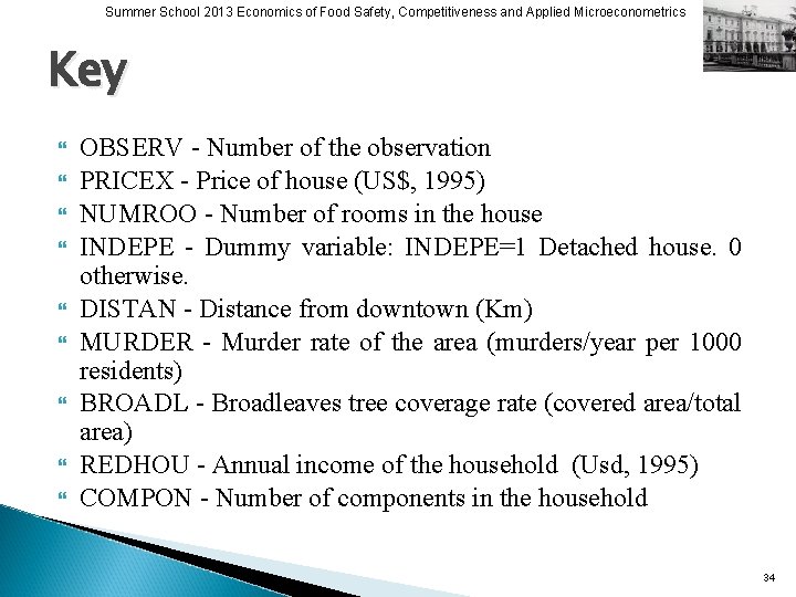
Summer School 2013 Economics of Food Safety, Competitiveness and Applied Microeconometrics Key OBSERV - Number of the observation PRICEX - Price of house (US$, 1995) NUMROO - Number of rooms in the house INDEPE - Dummy variable: INDEPE=1 Detached house. 0 otherwise. DISTAN - Distance from downtown (Km) MURDER - Murder rate of the area (murders/year per 1000 residents) BROADL - Broadleaves tree coverage rate (covered area/total area) REDHOU - Annual income of the household (Usd, 1995) COMPON - Number of components in the household 34

Trasformazione Box-Cox Summer School 2013 Economics of Food Safety, Competitiveness and Applied Microeconometrics

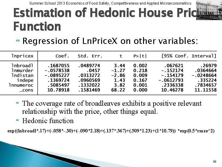
Summer School 2013 Economics of Food Safety, Competitiveness and Applied Microeconometrics Estimation of Hedonic House Price Function Regression of Ln. Price. X on other variables: The coverage rate of broadleaves exhibits a positive relevant relationship with the price, other things equal. Hedonic function exp((lnbroadl*. 17)+(-. 058*-. 30)+(-. 090*2. 18)+(. 137*. 367)+(. 509*1. 23)+(1*10. 79)) *exp(0. 5*rmse^2) 36

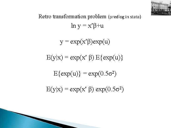
Retro transformation problem (predlog in stata) ln y = x’β+u y = exp(x’β)exp(u) E(y|x) = exp(x’ β) E{exp(u)} = exp(0. 5σ2) E(y|x) = exp(x’ β) exp(0. 5σ2)

Summer School 2013 Economics of Food Safety, Competitiveness and Applied Microeconometrics Estimation of Hedonic House Price Function Estimated Hedonic Price function is not linear: 38

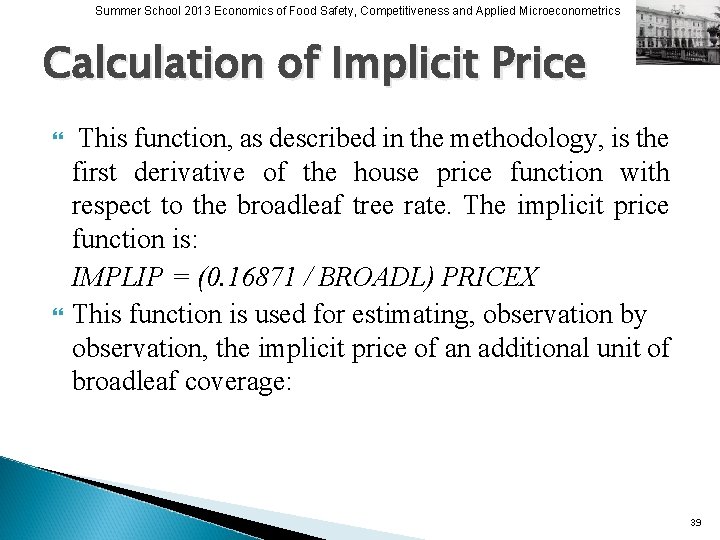
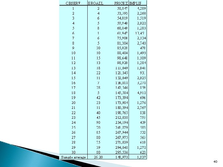
Summer School 2013 Economics of Food Safety, Competitiveness and Applied Microeconometrics Calculation of Implicit Price This function, as described in the methodology, is the first derivative of the house price function with respect to the broadleaf tree rate. The implicit price function is: IMPLIP = (0. 16871 / BROADL) PRICEX This function is used for estimating, observation by observation, the implicit price of an additional unit of broadleaf coverage: 39

40

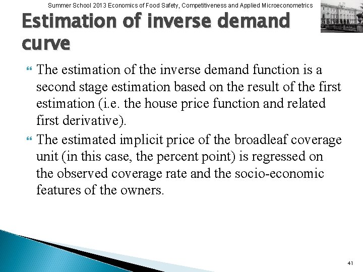
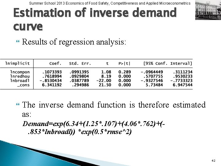
Summer School 2013 Economics of Food Safety, Competitiveness and Applied Microeconometrics Estimation of inverse demand curve The estimation of the inverse demand function is a second stage estimation based on the result of the first estimation (i. e. the house price function and related first derivative). The estimated implicit price of the broadleaf coverage unit (in this case, the percent point) is regressed on the observed coverage rate and the socio-economic features of the owners. 41

Summer School 2013 Economics of Food Safety, Competitiveness and Applied Microeconometrics Estimation of inverse demand curve Results of regression analysis: The inverse demand function is therefore estimated as: Demand=exp(6. 34+(1. 25*. 107)+(4. 06*. 762)+(. 853*lnbroadl)) *exp(0. 5*rmse^2) 42

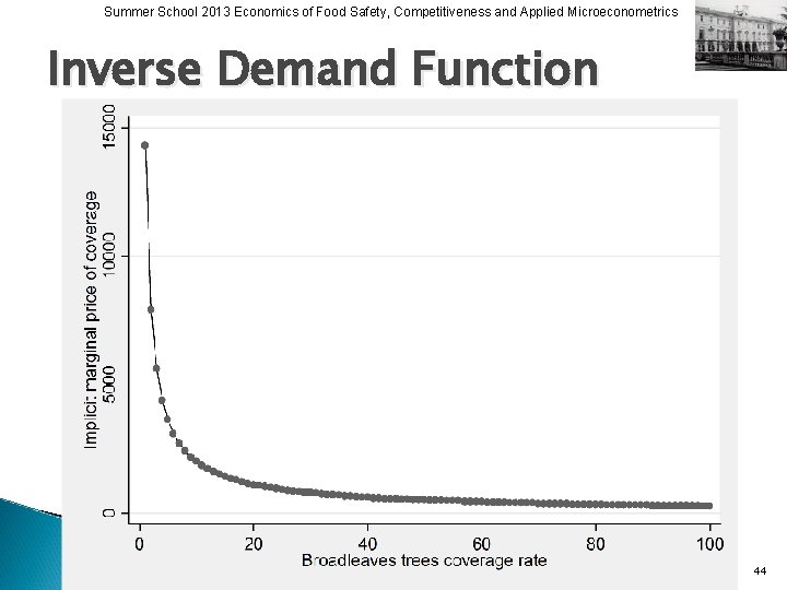
Summer School 2013 Economics of Food Safety, Competitiveness and Applied Microeconometrics Inverse Demand Function The inverse demand function can be shown. The variables COMPON REDHOU and are fixed at the sample mean level. 43

Summer School 2013 Economics of Food Safety, Competitiveness and Applied Microeconometrics Inverse Demand Function 44

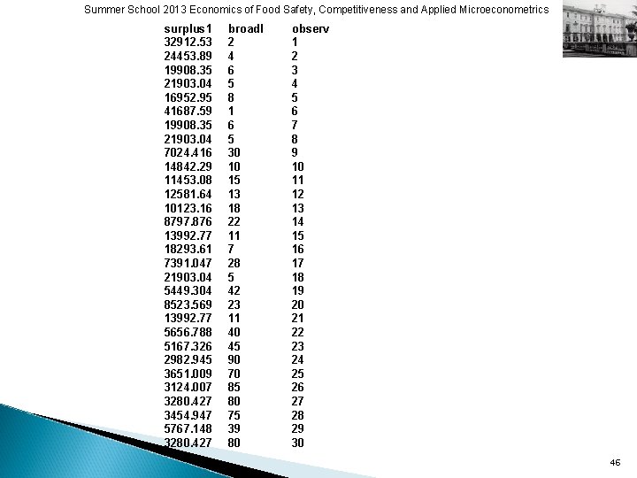
Summer School 2013 Economics of Food Safety, Competitiveness and Applied Microeconometrics Calculation of Consumer Surplus The consumer surplus is calculated by estimating the area under the demand curve. This is done by integrating the inverse demand curve with respect to the implicit price and calculating the definite integral observation by observation (between the present coverage rate (E 1=BROADL) and the coverage rate (new_broadl) planned by the policy maker (increase of 10% of the coverage) 45

Summer School 2013 Economics of Food Safety, Competitiveness and Applied Microeconometrics surplus 1 32912. 53 24453. 89 19908. 35 21903. 04 16952. 95 41687. 59 19908. 35 21903. 04 7024. 416 14842. 29 11453. 08 12581. 64 10123. 16 8797. 876 13992. 77 18293. 61 7391. 047 21903. 04 5449. 304 8523. 569 13992. 77 5656. 788 5167. 326 2982. 945 3651. 009 3124. 007 3280. 427 3454. 947 5767. 148 3280. 427 broadl 2 4 6 5 8 1 6 5 30 10 15 13 18 22 11 7 28 5 42 23 11 40 45 90 70 85 80 75 39 80 observ 1 2 3 4 5 6 7 8 9 10 11 12 13 14 15 16 17 18 19 20 21 22 23 24 25 26 27 28 29 30 46

Summer School 2013 Economics of Food Safety, Competitiveness and Applied Microeconometrics Discussion This information can be used first to calculate the average consumer surplus per household and can be multiplied by the number of households to get a measure of the total benefits which can be compared with the cost of the intervention. On distributional grounds, notice that a 10% increase for people living in areas with high coverage rate does not change the consumer surplus much, compared to those living in low coverage rate areas. 47