Fo PPS Summer school Solving Temporal Credit Assignment

Fo. PPS Summer school Solving Temporal Credit Assignment Doina Precup Mc. Gill University and Google Deep. Mind Montreal dprecup@cs. mcgill. ca Slides edited from Rich Sutton and Andy Barto’s presentations for ``Reinforcement Learning: An Introduction (2 nd ed. ) With thanks to Rich Sutton and the Reasoning & Learning Lab

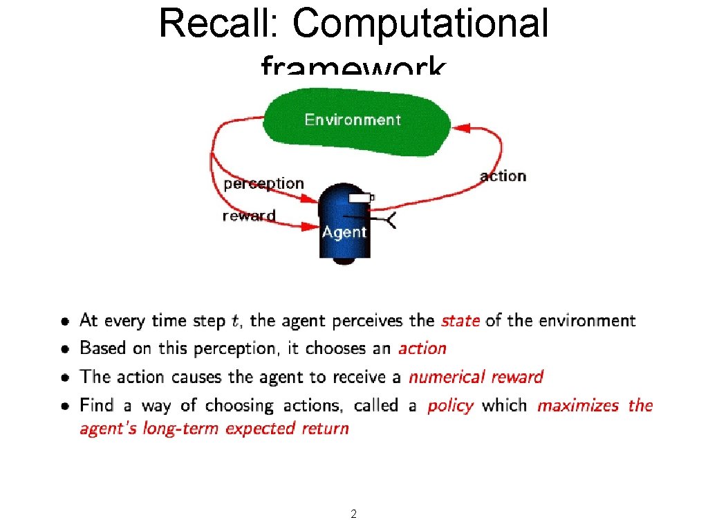
Recall: Computational framework 2

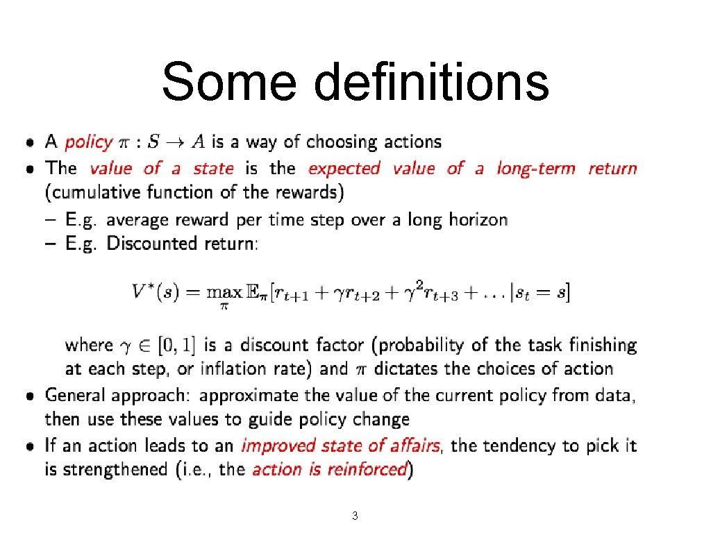
Some definitions 3

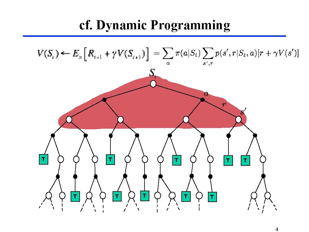
cf. Dynamic Programming T TT TT T T T 4

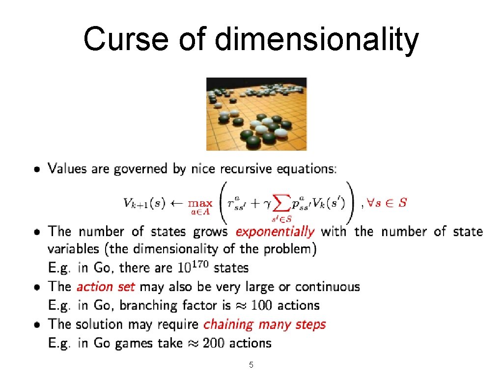
Curse of dimensionality 5

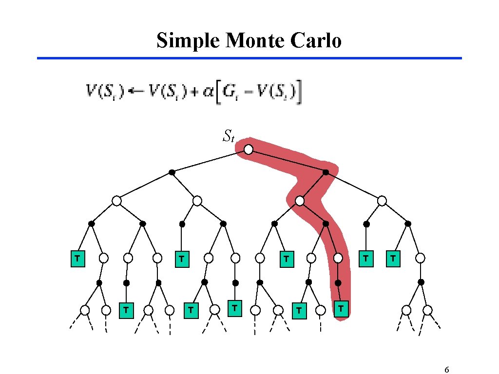
Simple Monte Carlo St T T TT T T TT 6

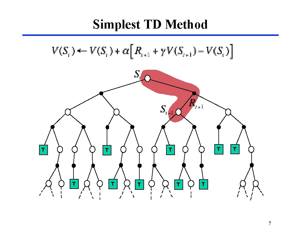
Simplest TD Method TT T T TT 7

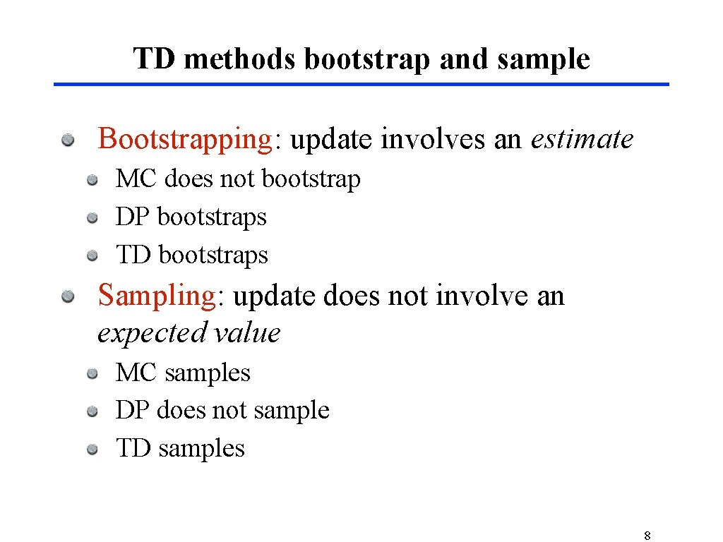
TD methods bootstrap and sample Bootstrapping: update involves an estimate MC does not bootstrap DP bootstraps TD bootstraps Sampling: update does not involve an expected value MC samples DP does not sample TD samples 8

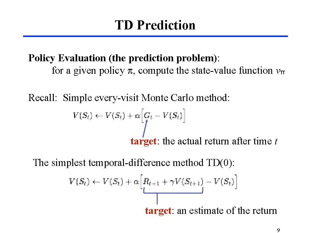
TD Prediction Policy Evaluation (the prediction problem): for a given policy p, compute the state-value function vπ Recall: Simple every-visit Monte Carlo method: target: the actual return after time t The simplest temporal-difference method TD(0): target: an estimate of the return 9

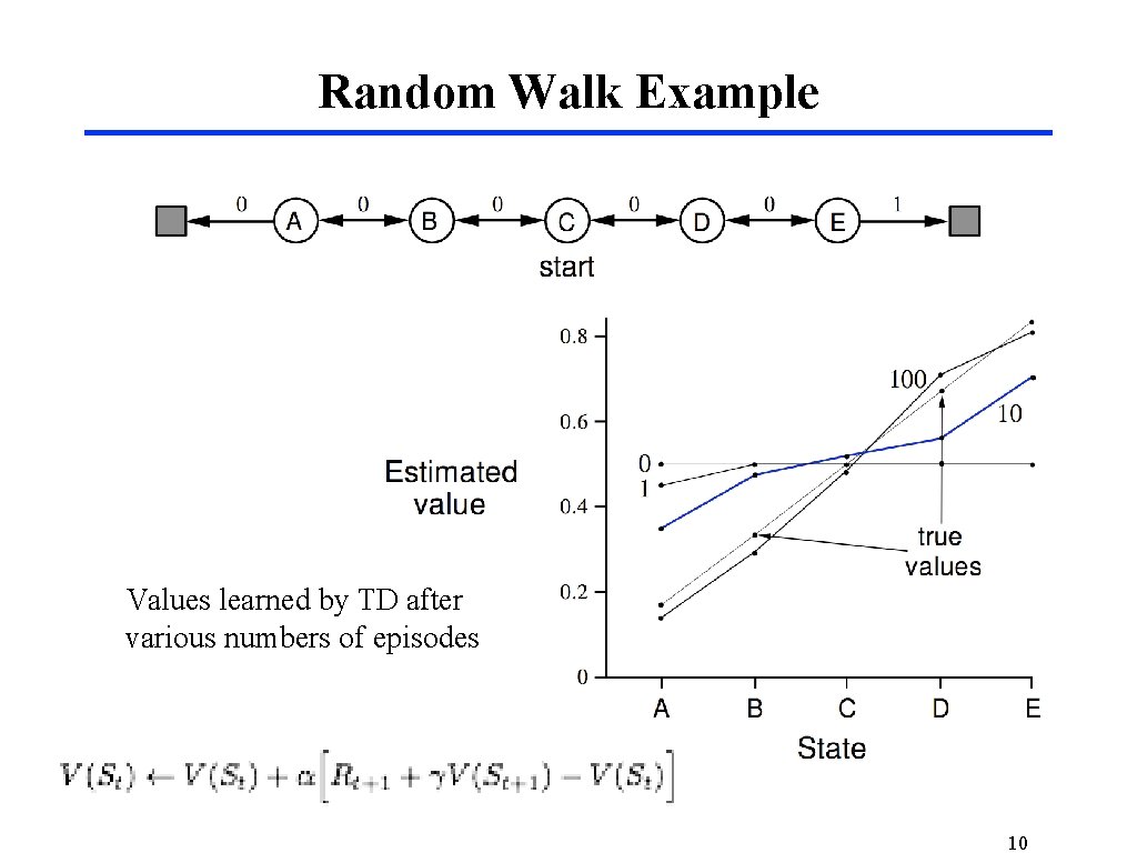
Random Walk Example Values learned by TD after various numbers of episodes 10

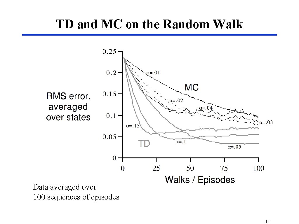
TD and MC on the Random Walk Data averaged over 100 sequences of episodes 11

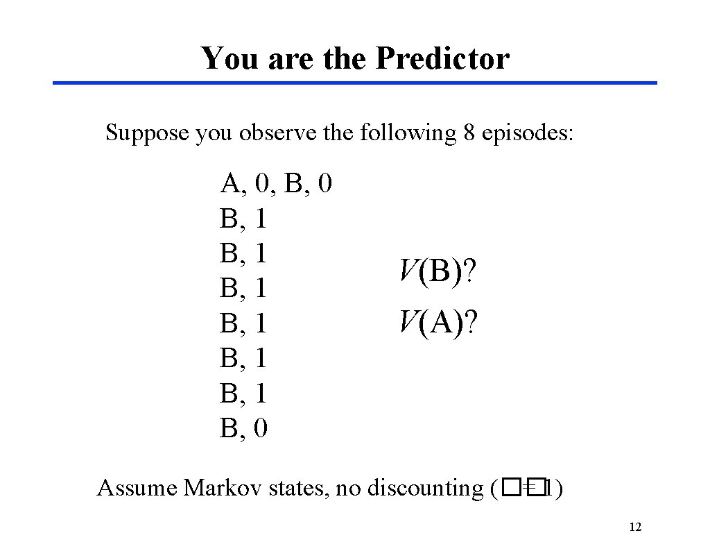
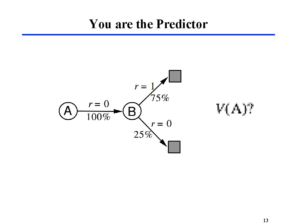
You are the Predictor Suppose you observe the following 8 episodes: A, 0, B, 0 B, 1 B, 1 B, 0 V(B)? V(A)? Assume Markov states, no discounting (�� = 1) 12

You are the Predictor 13

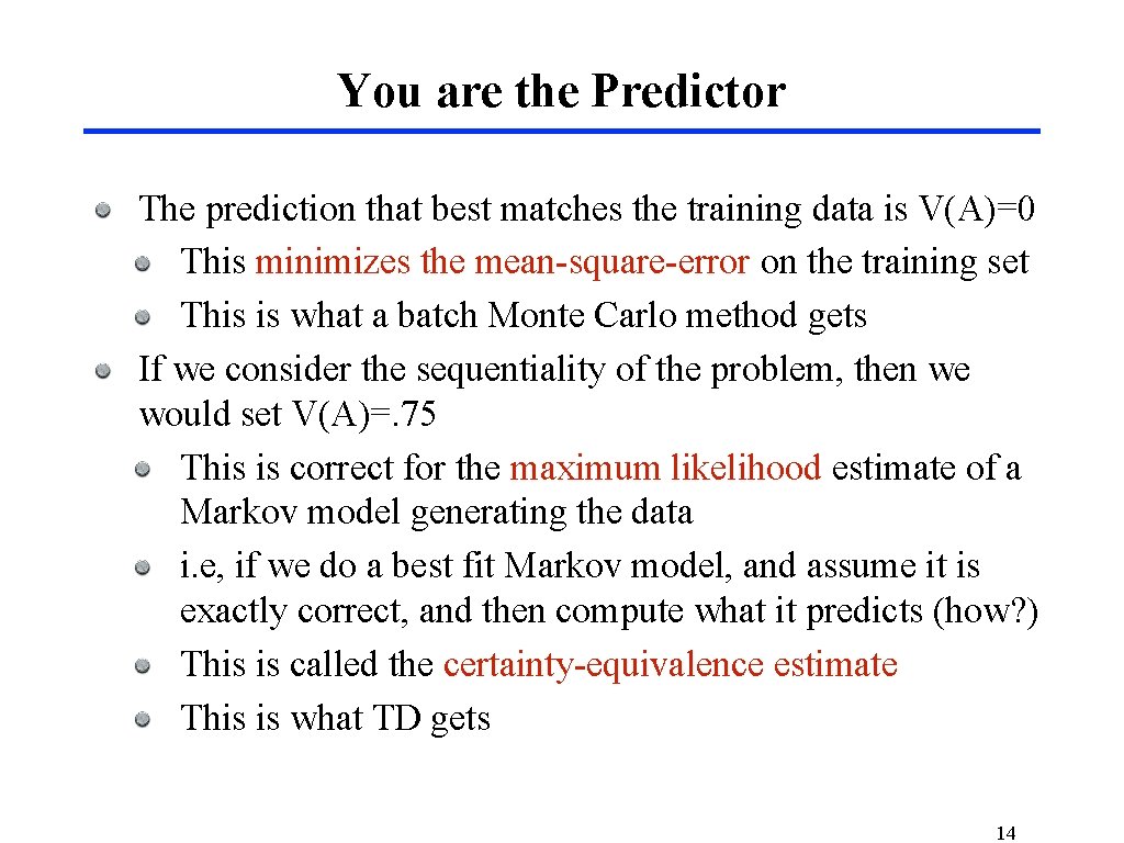
You are the Predictor The prediction that best matches the training data is V(A)=0 This minimizes the mean-square-error on the training set This is what a batch Monte Carlo method gets If we consider the sequentiality of the problem, then we would set V(A)=. 75 This is correct for the maximum likelihood estimate of a Markov model generating the data i. e, if we do a best fit Markov model, and assume it is exactly correct, and then compute what it predicts (how? ) This is called the certainty-equivalence estimate This is what TD gets 14

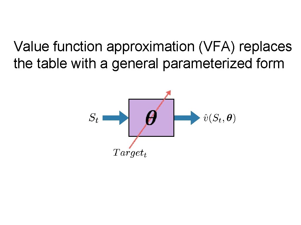
Value function approximation (VFA) replaces the table with a general parameterized form

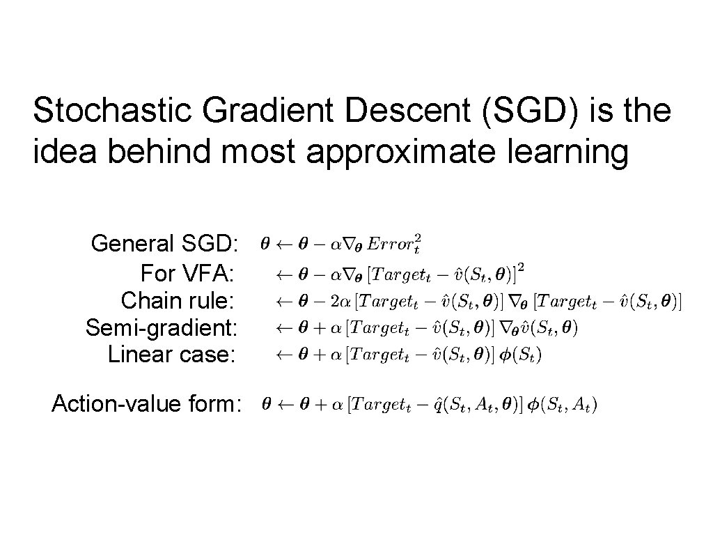
Stochastic Gradient Descent (SGD) is the idea behind most approximate learning General SGD: For VFA: Chain rule: Semi-gradient: Linear case: Action-value form:

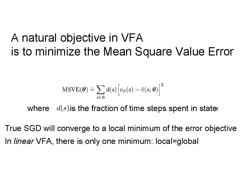
A natural objective in VFA is to minimize the Mean Square Value Error where is the fraction of time steps spent in state True SGD will converge to a local minimum of the error objective In linear VFA, there is only one minimum: local=global

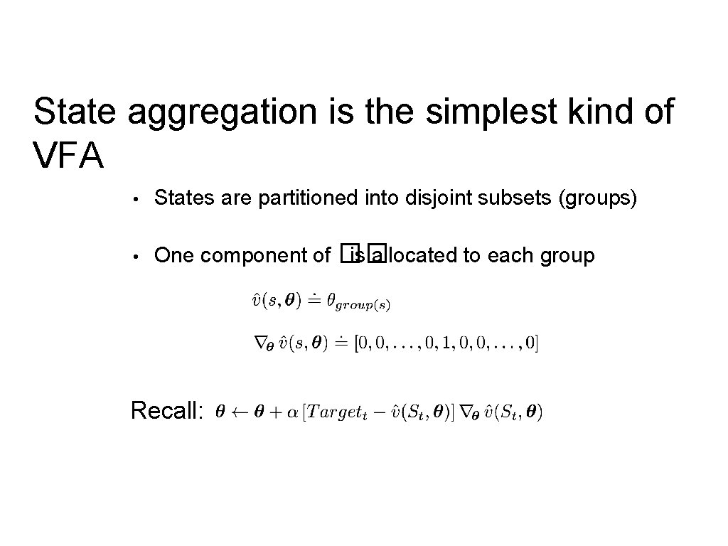
State aggregation is the simplest kind of VFA • States are partitioned into disjoint subsets (groups) • One component of �� is allocated to each group Recall:

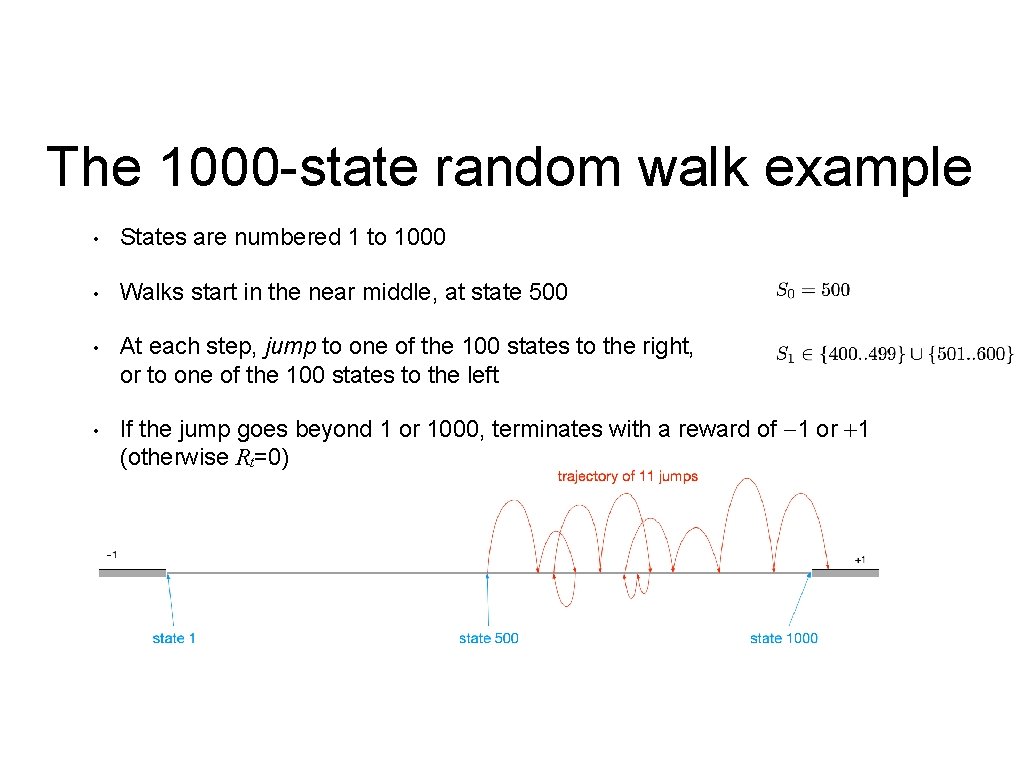
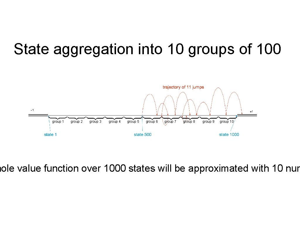
The 1000 -state random walk example • States are numbered 1 to 1000 • Walks start in the near middle, at state 500 • At each step, jump to one of the 100 states to the right, or to one of the 100 states to the left • If the jump goes beyond 1 or 1000, terminates with a reward of -1 or +1 (otherwise Rt=0)

State aggregation into 10 groups of 100 group 1 group 2 group 3 group 4 group 5 group 6 group 7 group 8 group 9 group 10 hole value function over 1000 states will be approximated with 10 num

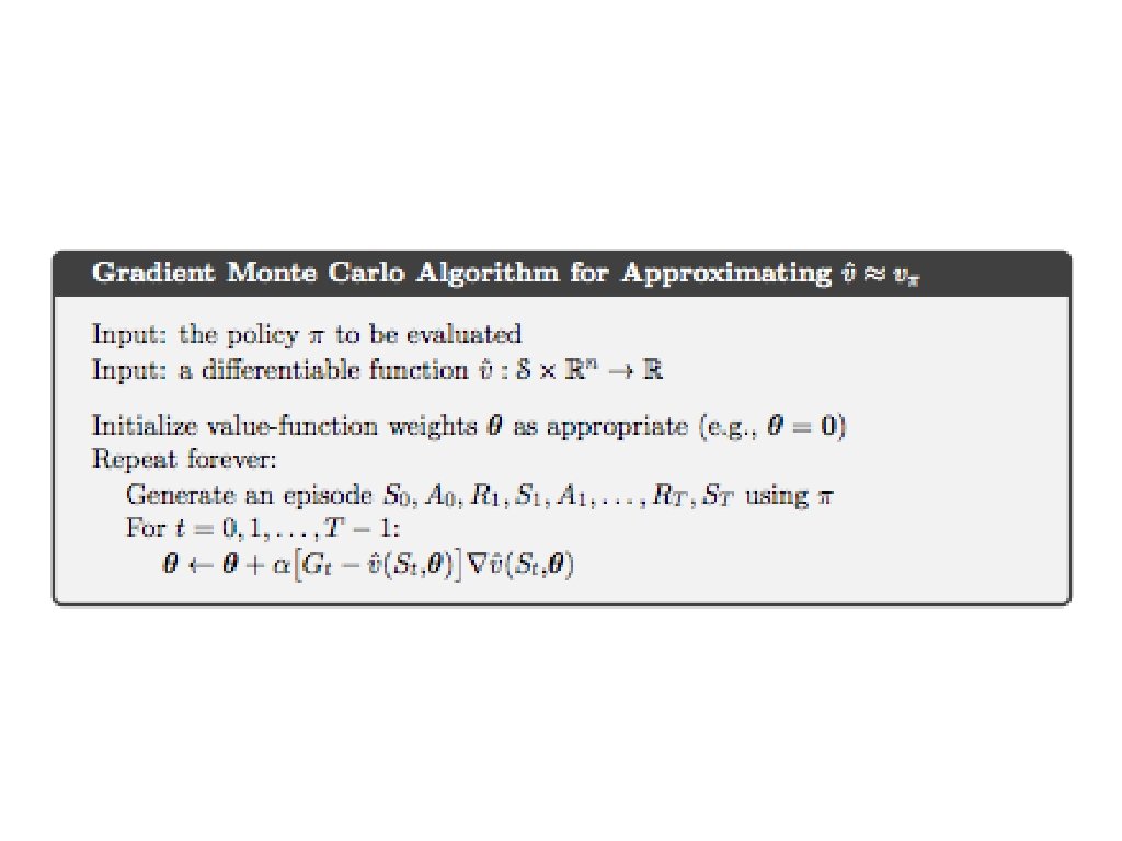
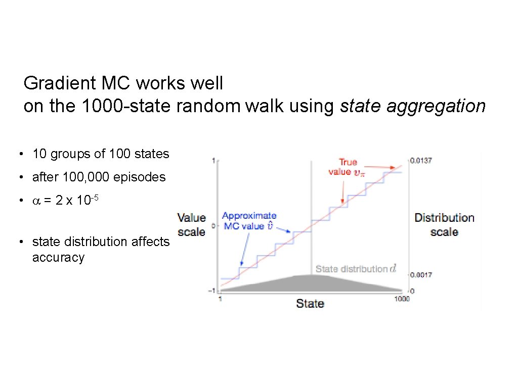
Gradient MC works well on the 1000 -state random walk using state aggregation • 10 groups of 100 states • after 100, 000 episodes • a = 2 x 10 -5 • state distribution affects accuracy

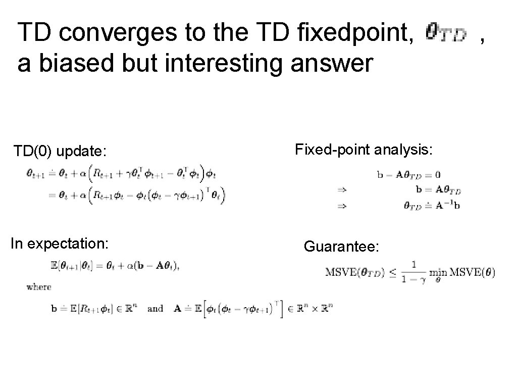
TD converges to the TD fixedpoint, a biased but interesting answer TD(0) update: In expectation: Fixed-point analysis: Guarantee: ,

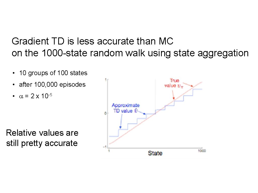
Gradient TD is less accurate than MC on the 1000 -state random walk using state aggregation • 10 groups of 100 states • after 100, 000 episodes • a = 2 x 10 -5 Relative values are still pretty accurate

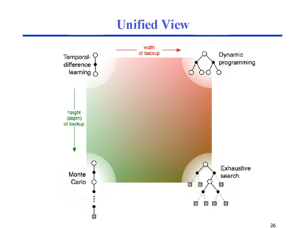
Unified View 26

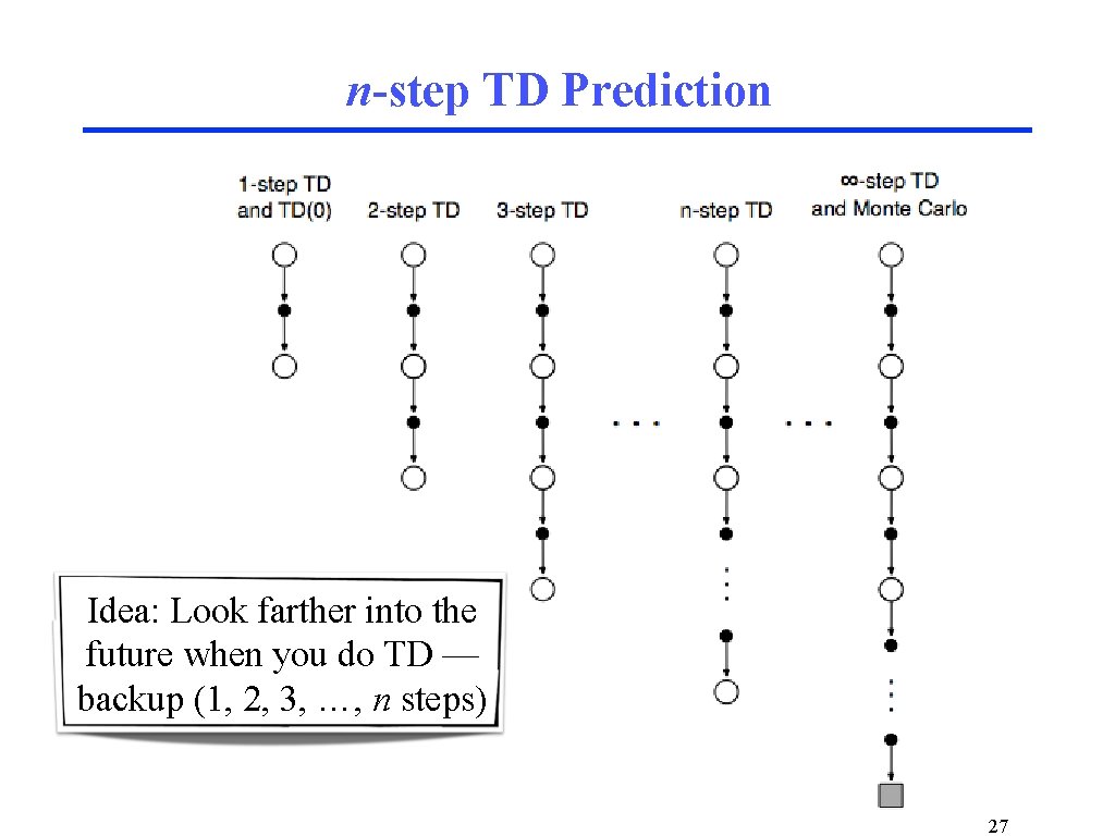
n-step TD Prediction Idea: Look farther into the future when you do TD — backup (1, 2, 3, …, n steps) 27

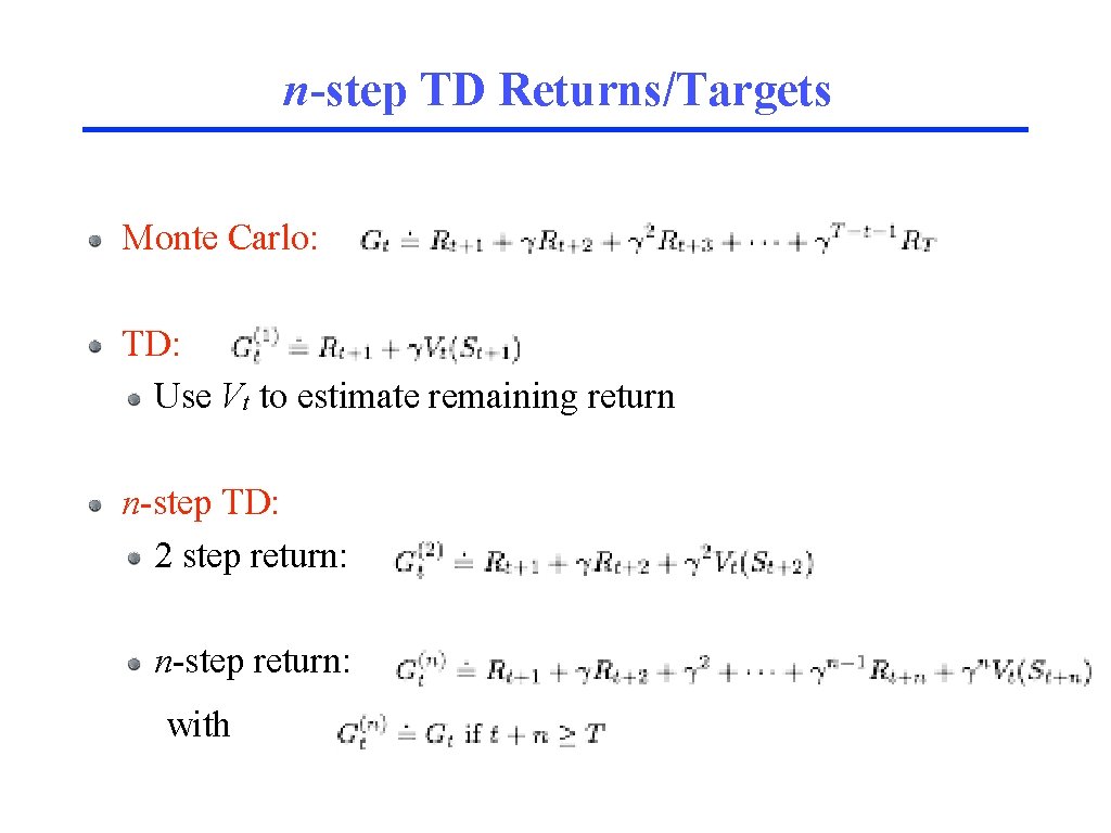
n-step TD Returns/Targets Monte Carlo: TD: Use Vt to estimate remaining return n-step TD: 2 step return: n-step return: with

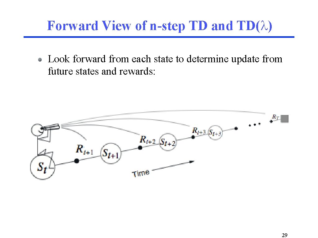
Forward View of n-step TD and TD(l) Look forward from each state to determine update from future states and rewards: 29

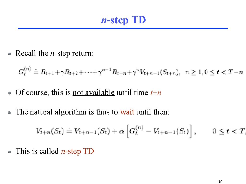
n-step TD Recall the n-step return: Of course, this is not available until time t+n The natural algorithm is thus to wait until then: This is called n-step TD 30

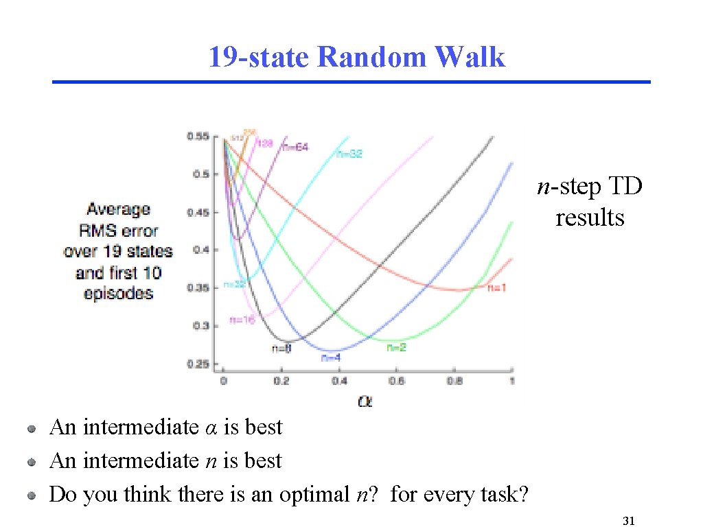
19 -state Random Walk n-step TD results An intermediate α is best An intermediate n is best Do you think there is an optimal n? for every task? 31

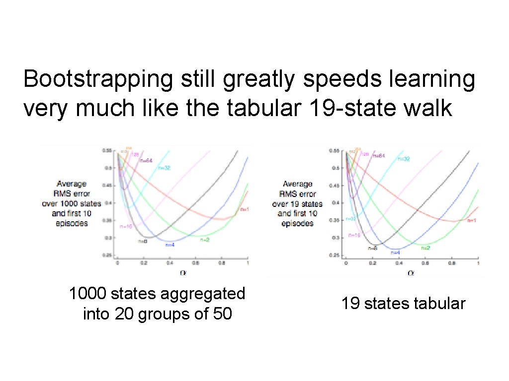
Bootstrapping still greatly speeds learning very much like the tabular 19 -state walk 1000 states aggregated into 20 groups of 50 19 states tabular

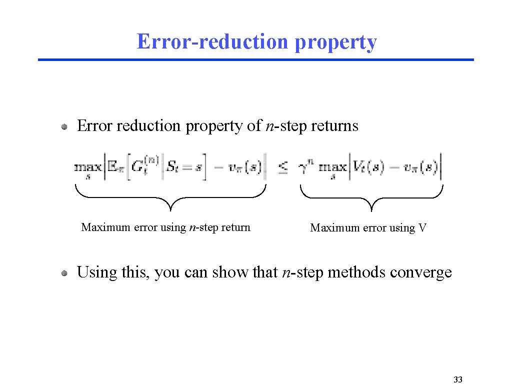
Error-reduction property Error reduction property of n-step returns Maximum error using n-step return Maximum error using V Using this, you can show that n-step methods converge 33

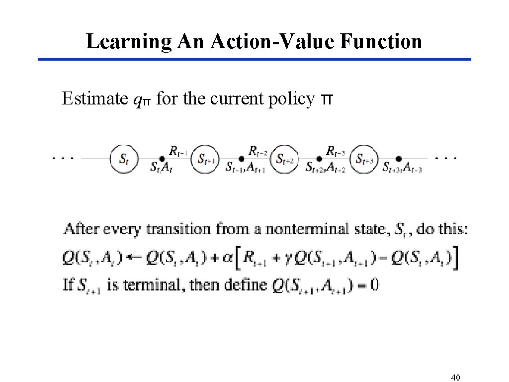
Learning An Action-Value Function Estimate qπ for the current policy π 40

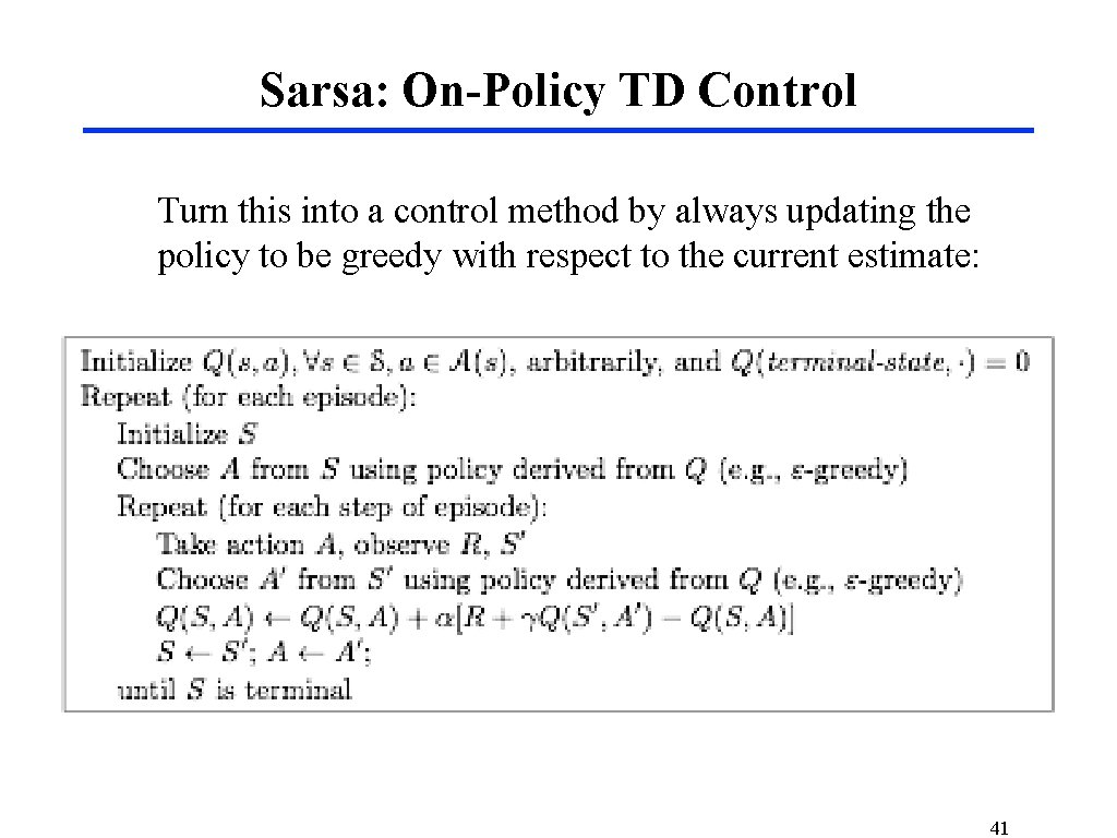
Sarsa: On-Policy TD Control Turn this into a control method by always updating the policy to be greedy with respect to the current estimate: 41

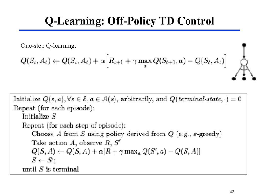
Q-Learning: Off-Policy TD Control One-step Q-learning: 42

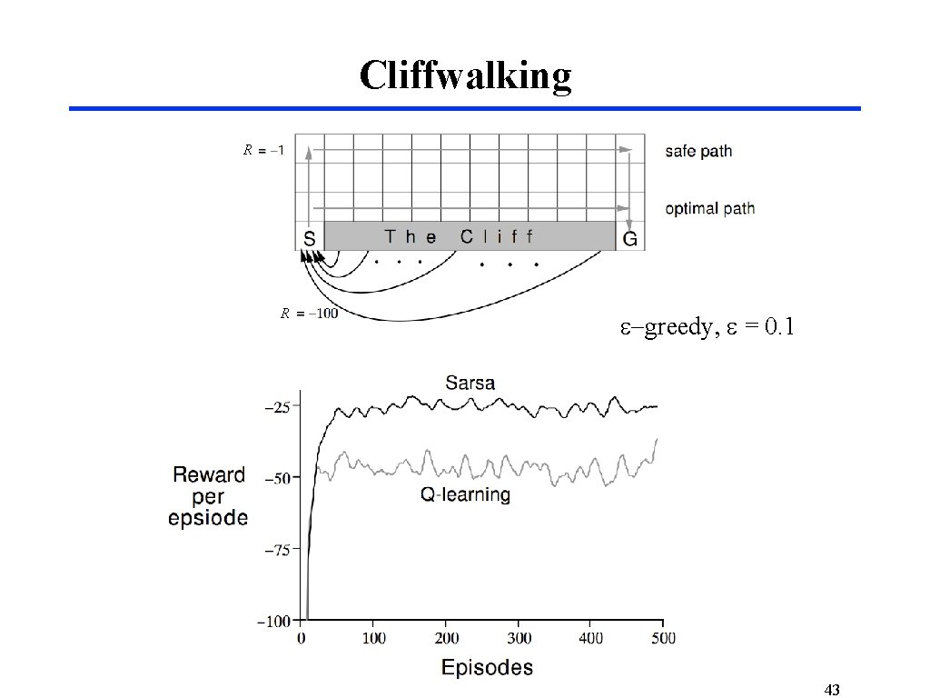
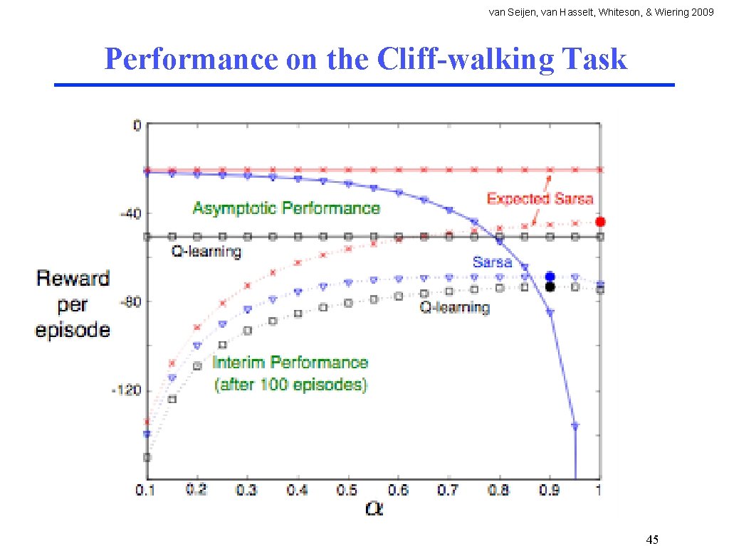
Cliffwalking R R e-greedy, e = 0. 1 43

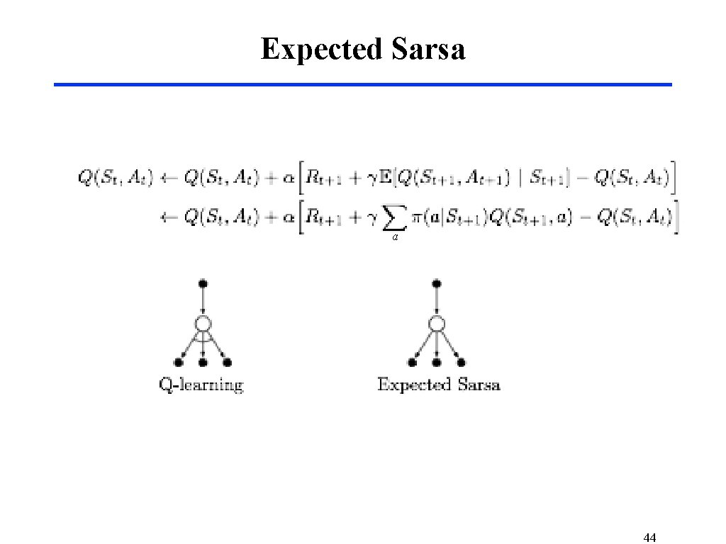
Expected Sarsa a 44

van Seijen, van Hasselt, Whiteson, & Wiering 2009 Performance on the Cliff-walking Task 45

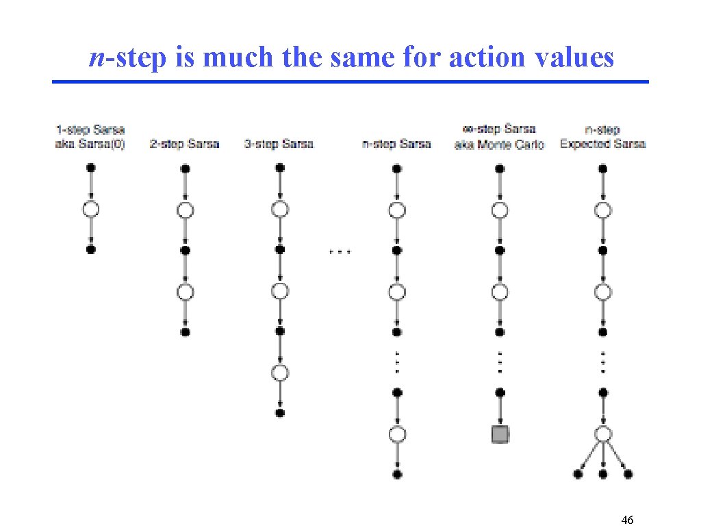
n-step is much the same for action values 46

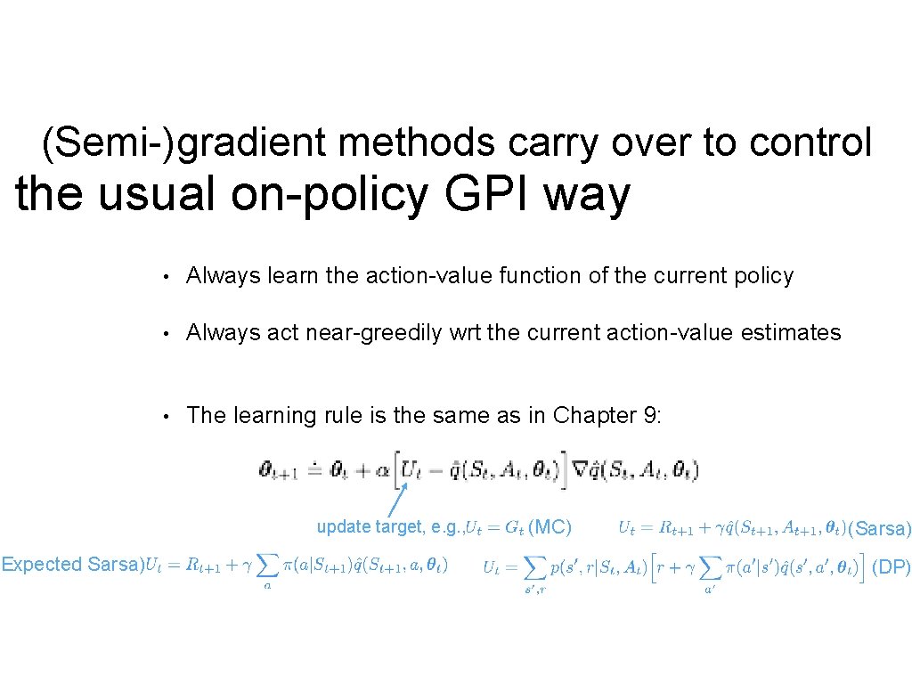
(Semi-)gradient methods carry over to control n the usual on-policy GPI way (Expected Sarsa) • Always learn the action-value function of the current policy • Always act near-greedily wrt the current action-value estimates • The learning rule is the same as in Chapter 9: update target, e. g. , (MC) (Sarsa) (DP)

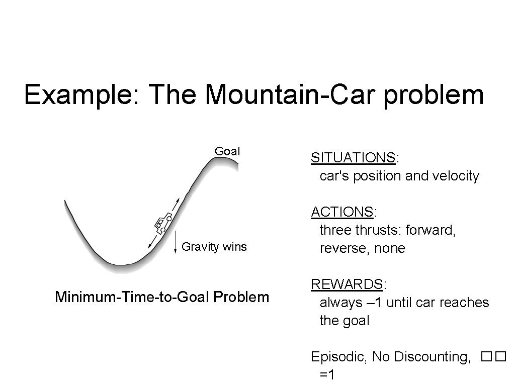
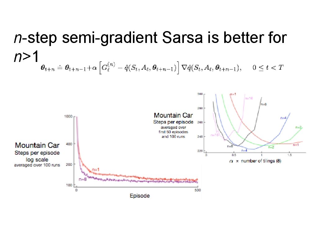
Example: The Mountain-Car problem Goal Gravity wins Minimum-Time-to-Goal Problem SITUATIONS: car's position and velocity ACTIONS: three thrusts: forward, reverse, none REWARDS: always – 1 until car reaches the goal Episodic, No Discounting, �� =1

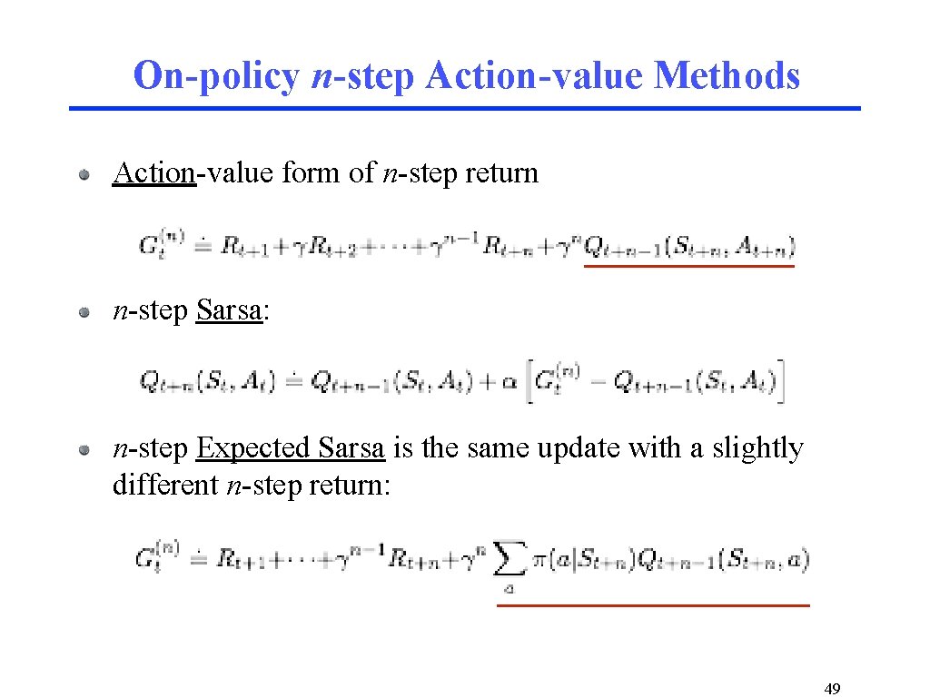
On-policy n-step Action-value Methods Action-value form of n-step return n-step Sarsa: n-step Expected Sarsa is the same update with a slightly different n-step return: 49

n-step semi-gradient Sarsa is better for n>1

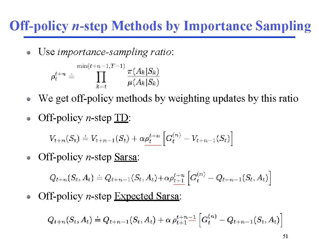
Off-policy n-step Methods by Importance Sampling Use importance-sampling ratio: We get off-policy methods by weighting updates by this ratio Off-policy n-step TD: Off-policy n-step Sarsa: Off-policy n-step Expected Sarsa: 51

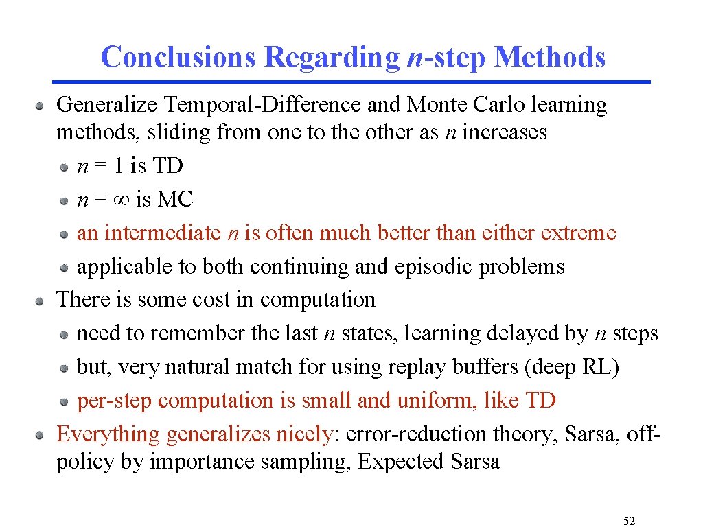
Conclusions Regarding n-step Methods Generalize Temporal-Difference and Monte Carlo learning methods, sliding from one to the other as n increases n = 1 is TD n = ∞ is MC an intermediate n is often much better than either extreme applicable to both continuing and episodic problems There is some cost in computation need to remember the last n states, learning delayed by n steps but, very natural match for using replay buffers (deep RL) per-step computation is small and uniform, like TD Everything generalizes nicely: error-reduction theory, Sarsa, offpolicy by importance sampling, Expected Sarsa 52

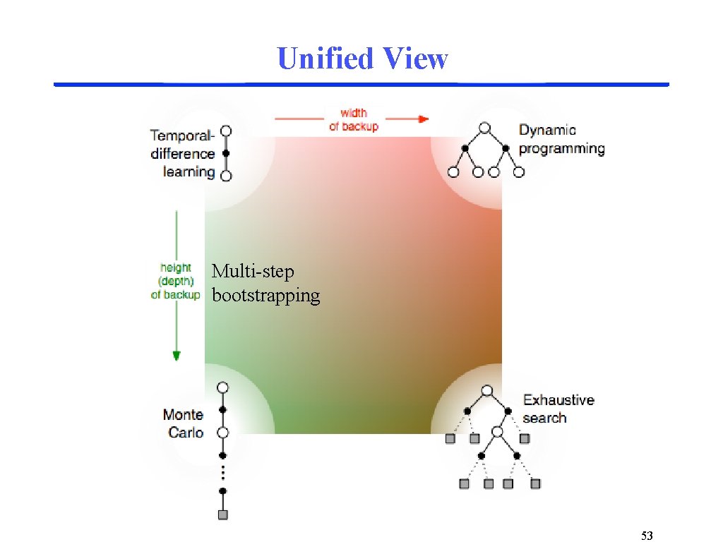
Unified View Multi-step bootstrapping 53

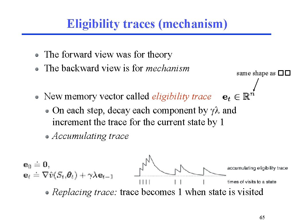
Eligibility traces are: Another way of interpolating between MC and TD methods A way of implementing compound λ-return targets A basic mechanistic idea — a short-term, fading memory A new style of algorithm development/analysis the forward-view ⇔ backward-view transformation Forward view: conceptually simple — good for theory, intuition Backward view: computational implementation of the forward view 54

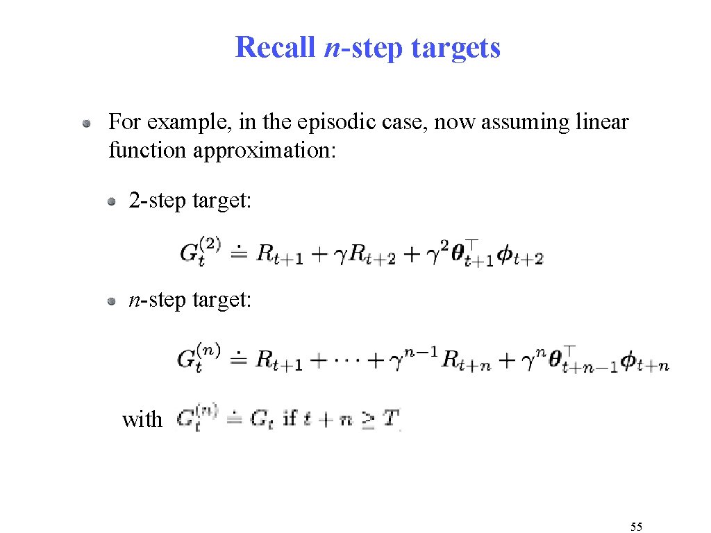
Recall n-step targets For example, in the episodic case, now assuming linear function approximation: 2 -step target: n-step target: with 55

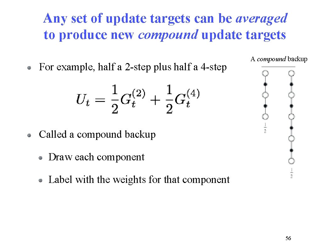
Any set of update targets can be averaged to produce new compound update targets For example, half a 2 -step plus half a 4 -step A compound backup Called a compound backup Draw each component Label with the weights for that component 56

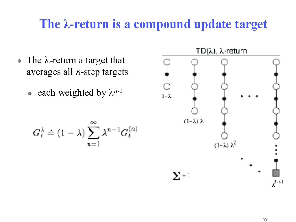
The λ-return is a compound update target The l-return a target that averages all n-step targets each weighted by ln-1 57

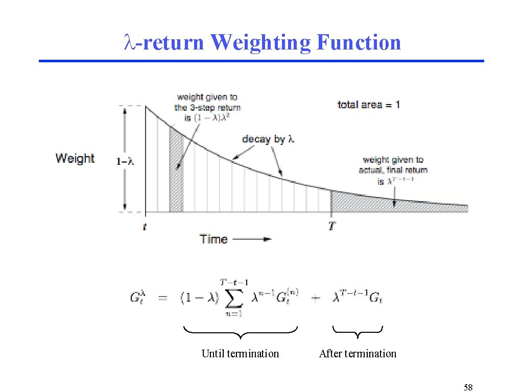
l-return Weighting Function Until termination After termination 58

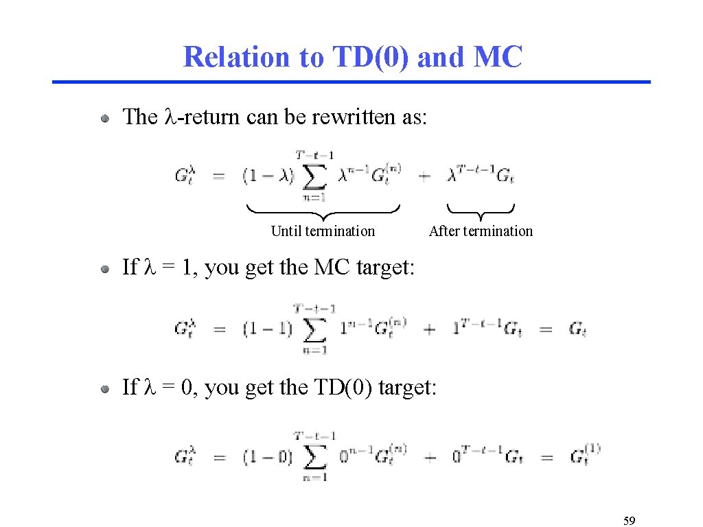
Relation to TD(0) and MC The l-return can be rewritten as: Until termination After termination If l = 1, you get the MC target: If l = 0, you get the TD(0) target: 59

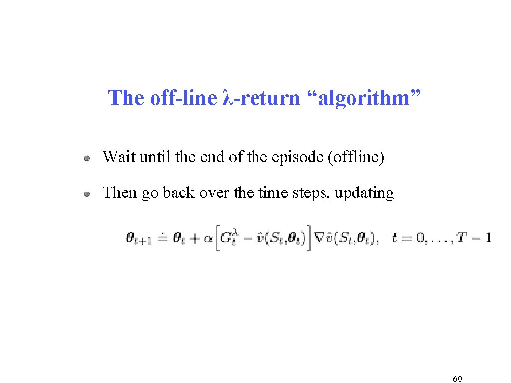
The off-line λ-return “algorithm” Wait until the end of the episode (offline) Then go back over the time steps, updating 60

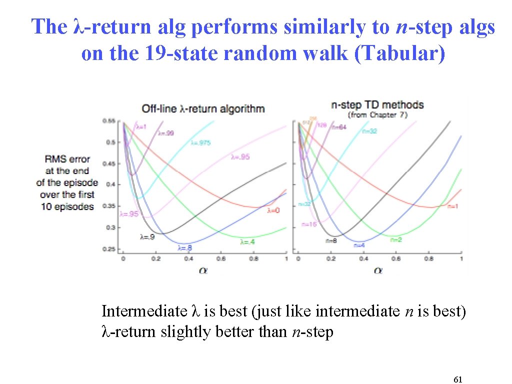
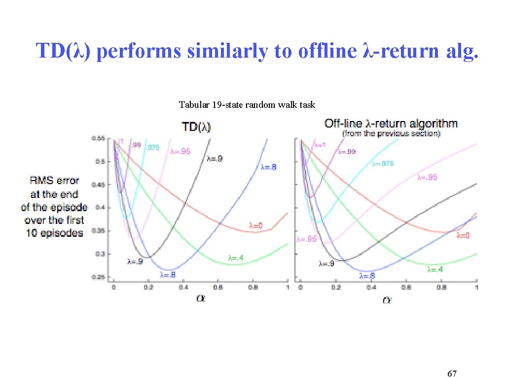
The λ-return alg performs similarly to n-step algs on the 19 -state random walk (Tabular) Intermediate λ is best (just like intermediate n is best) λ-return slightly better than n-step 61

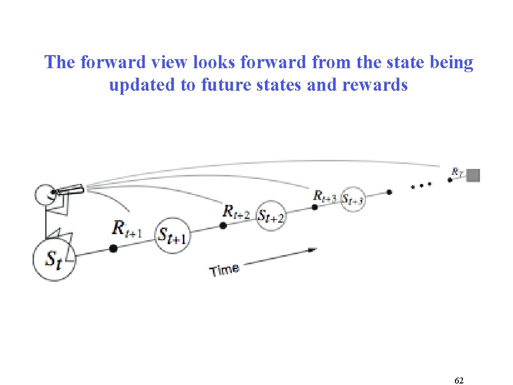
The forward view looks forward from the state being updated to future states and rewards 62

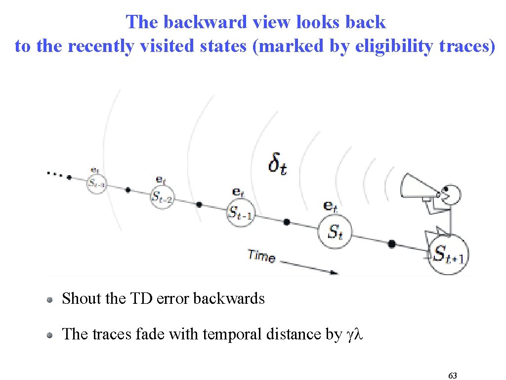
The backward view looks back to the recently visited states (marked by eligibility traces) Shout the TD error backwards The traces fade with temporal distance by gl 63

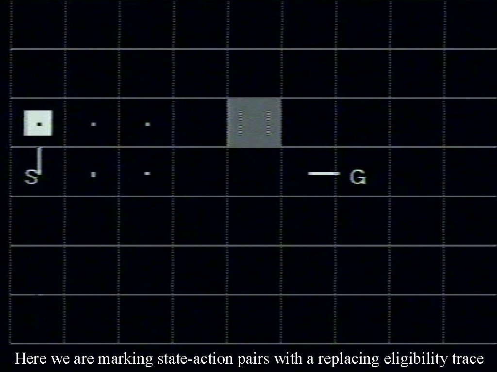
Demo Here we are marking state-action pairs with a replacing eligibility 64 trace

Eligibility traces (mechanism) The forward view was for theory The backward view is for mechanism same shape as �� New memory vector called eligibility trace On each step, decay each component by gl and increment the trace for the current state by 1 Accumulating trace Replacing trace: trace becomes 1 when state is visited 65

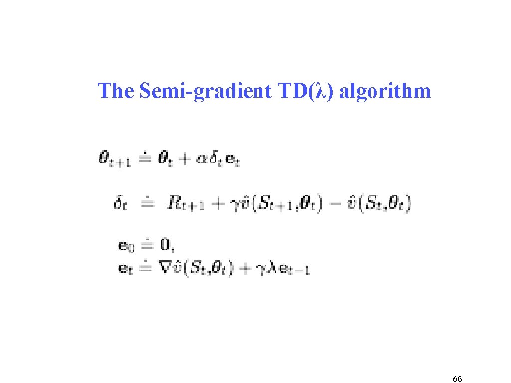
The Semi-gradient TD(λ) algorithm 66

TD(λ) performs similarly to offline λ-return alg. Tabular 19 -state random walk task 67

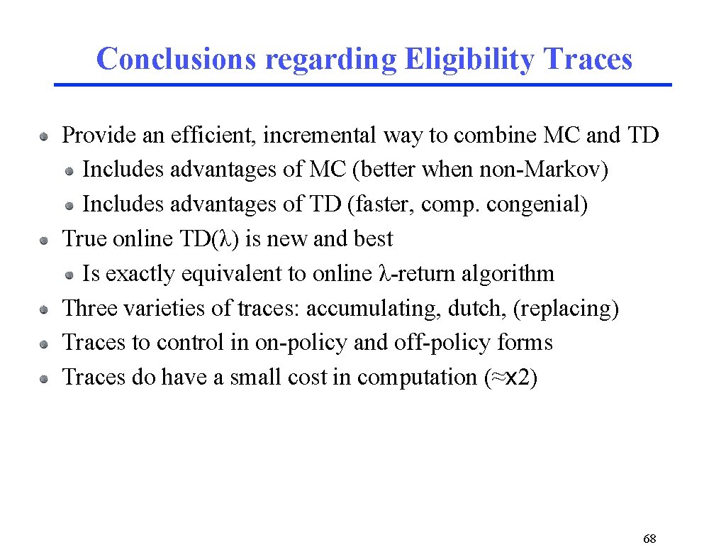
Conclusions regarding Eligibility Traces Provide an efficient, incremental way to combine MC and TD Includes advantages of MC (better when non-Markov) Includes advantages of TD (faster, comp. congenial) True online TD(λ) is new and best Is exactly equivalent to online λ-return algorithm Three varieties of traces: accumulating, dutch, (replacing) Traces to control in on-policy and off-policy forms Traces do have a small cost in computation (≈x 2) 68

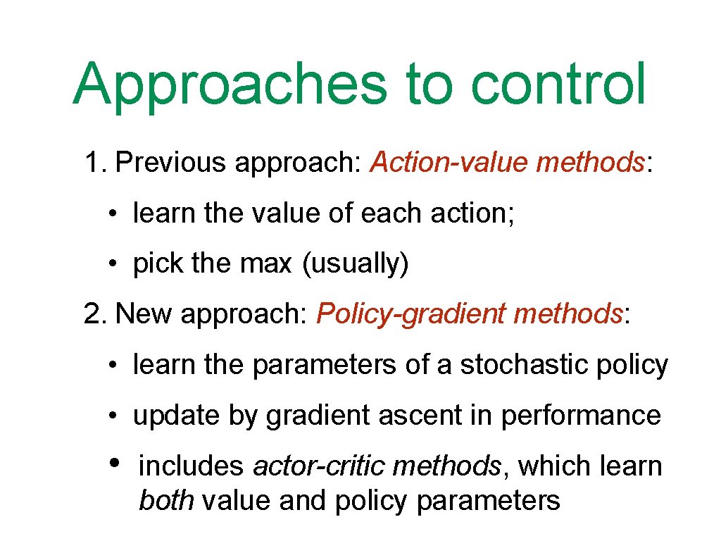
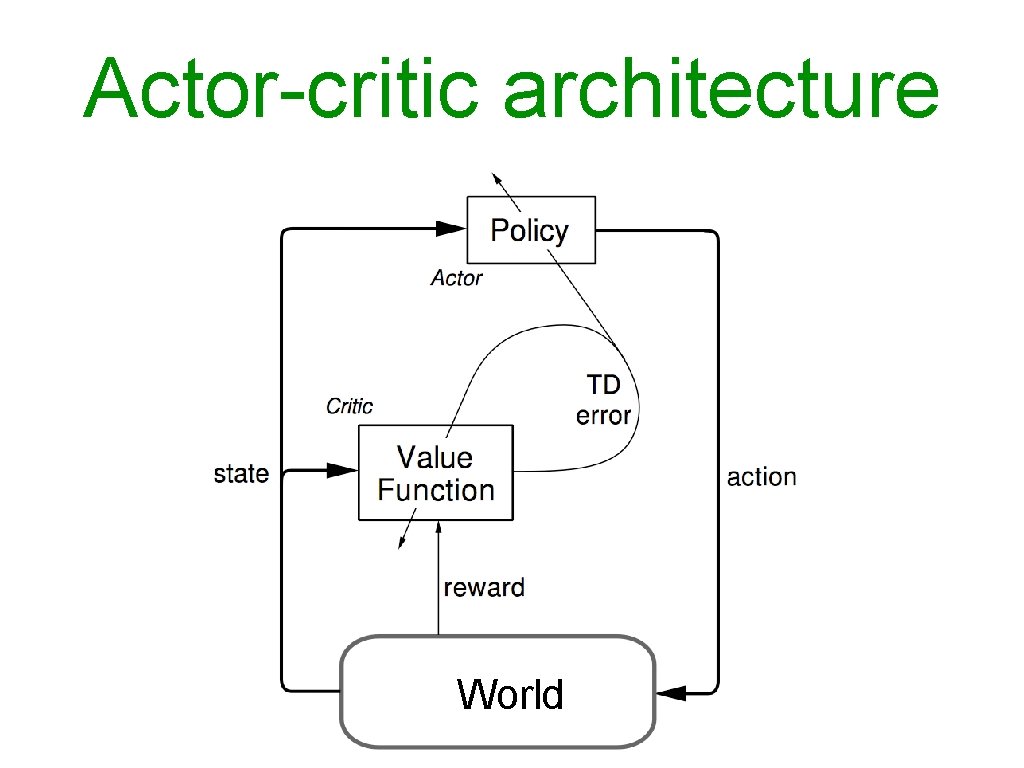
Approaches to control 1. Previous approach: Action-value methods: • learn the value of each action; • pick the max (usually) 2. New approach: Policy-gradient methods: • learn the parameters of a stochastic policy • update by gradient ascent in performance • includes actor-critic methods, which learn both value and policy parameters

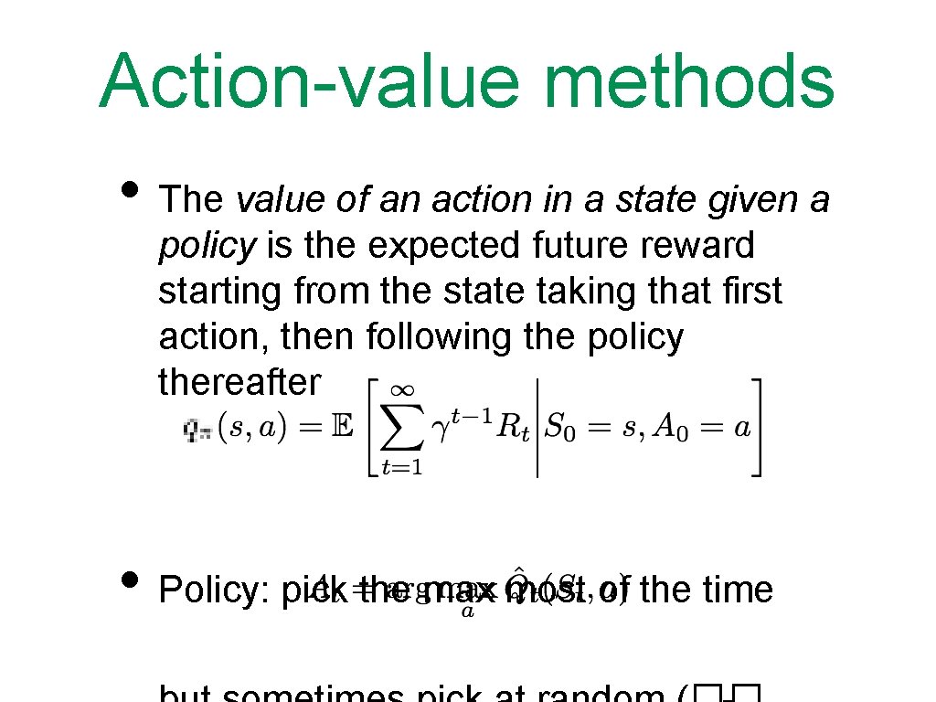
Action-value methods • The value of an action in a state given a policy is the expected future reward starting from the state taking that first action, then following the policy thereafter • Policy: pick the max most of the time

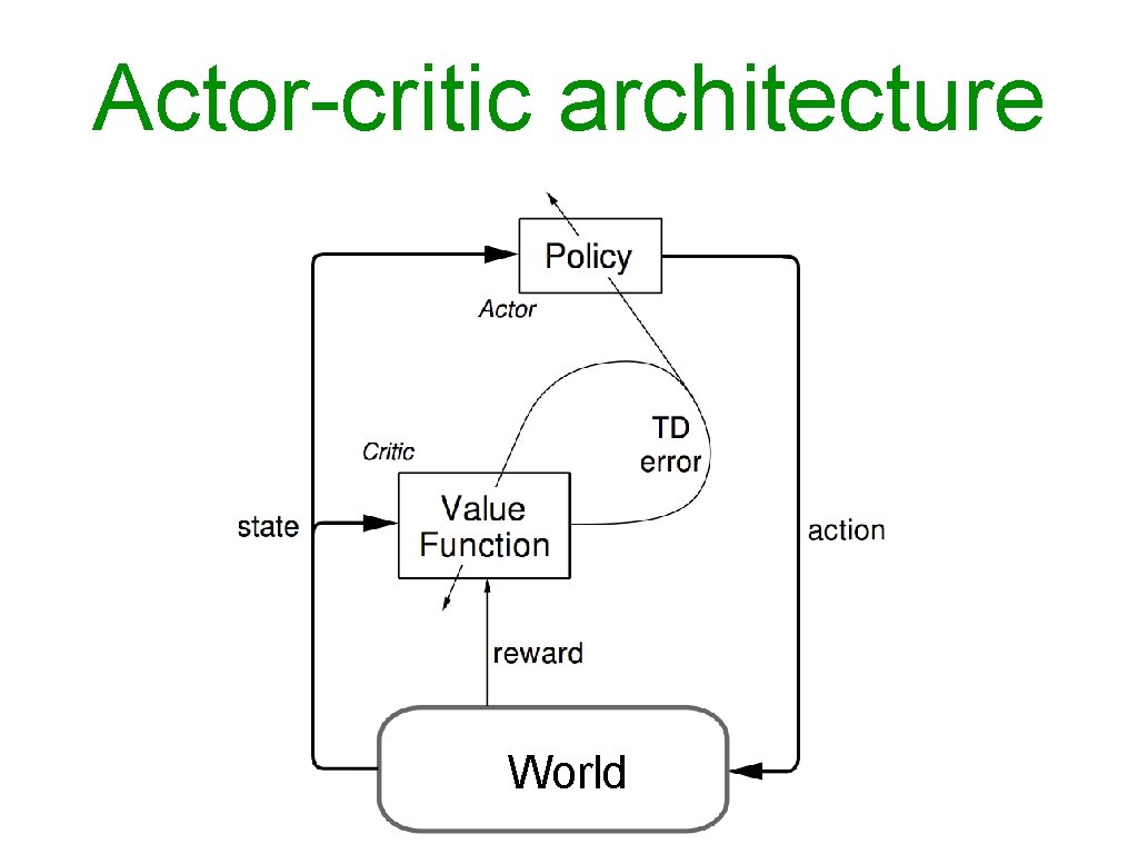
Actor-critic architecture World

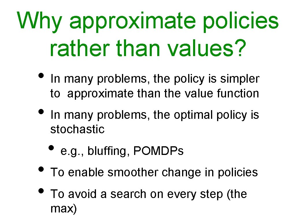
Why approximate policies rather than values? • In many problems, the policy is simpler to approximate than the value function • In many problems, the optimal policy is stochastic • e. g. , bluffing, POMDPs • To enable smoother change in policies • To avoid a search on every step (the max)

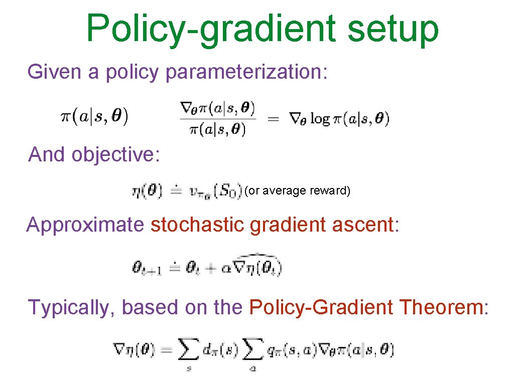
Policy-gradient setup Given a policy parameterization: And objective: (or average reward) Approximate stochastic gradient ascent: Typically, based on the Policy-Gradient Theorem:

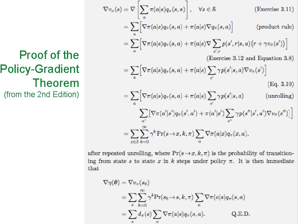
Proof of the Policy-Gradient Theorem (from the 2 nd Edition)

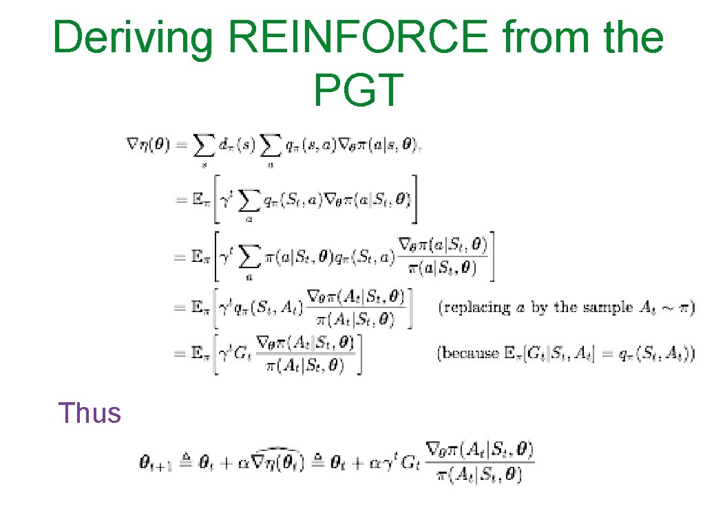
Deriving REINFORCE from the PGT Thus

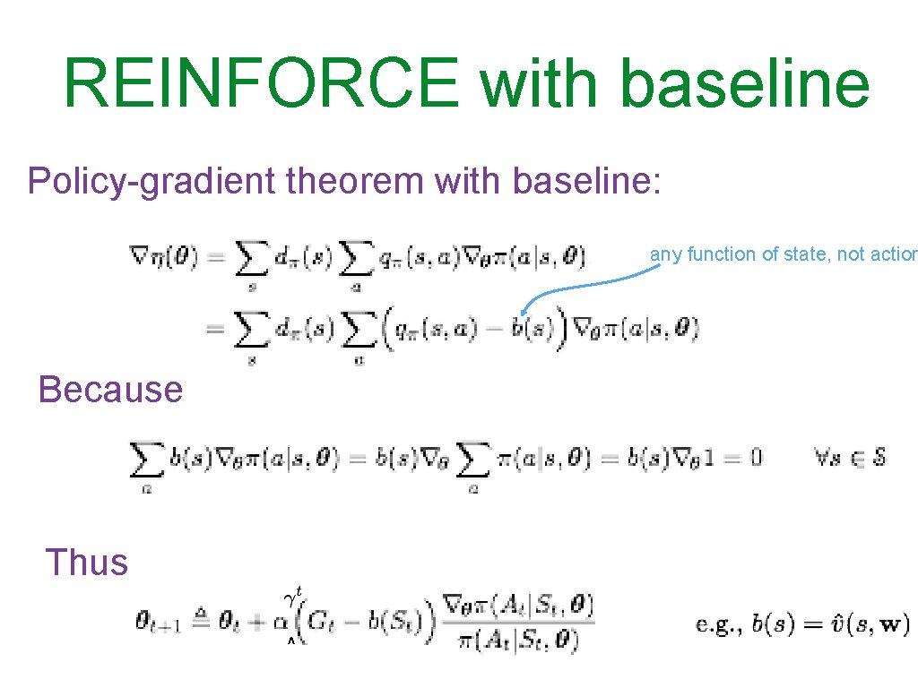
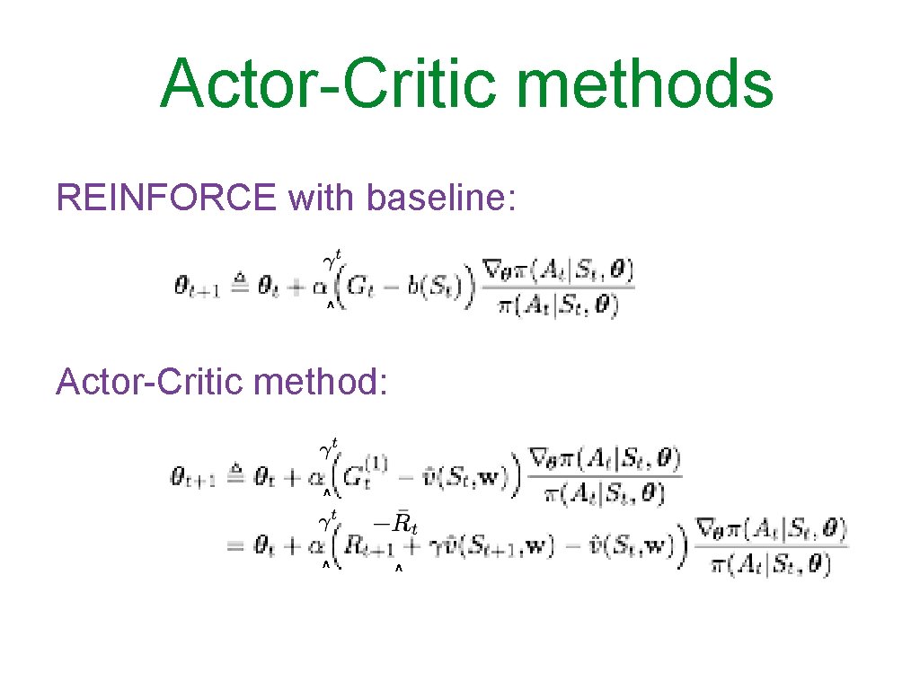
REINFORCE with baseline Policy-gradient theorem with baseline: any function of state, not action Because Thus ^

Actor-critic architecture World

Actor-Critic methods REINFORCE with baseline: ^ Actor-Critic method: ^ ^ ^

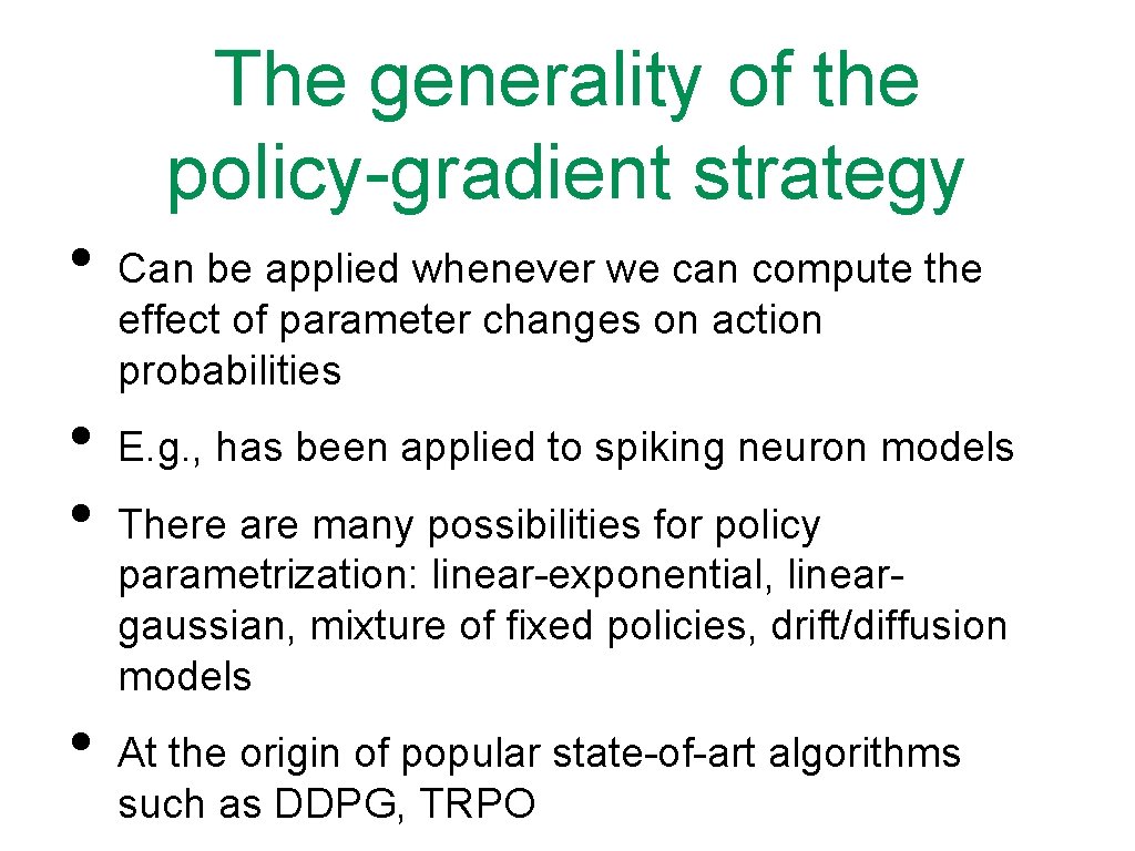
The generality of the policy-gradient strategy • • Can be applied whenever we can compute the effect of parameter changes on action probabilities E. g. , has been applied to spiking neuron models There are many possibilities for policy parametrization: linear-exponential, lineargaussian, mixture of fixed policies, drift/diffusion models At the origin of popular state-of-art algorithms such as DDPG, TRPO

Example: DDPG • https: //www. youtube. com/watch? v=i. Fg 5 lc. Uz. SYU