Wavelets Chapter 7 What are Wavelets Wavelets are

Wavelets (Chapter 7)

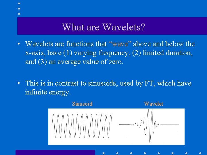
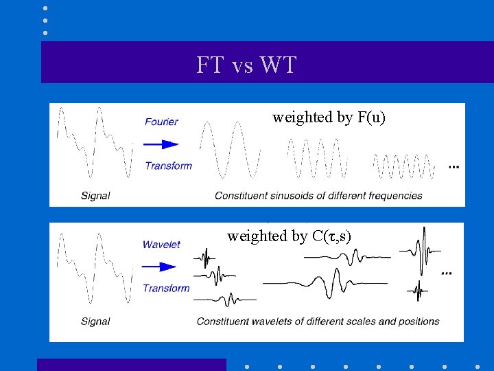
What are Wavelets? • Wavelets are functions that “wave” above and below the x-axis, have (1) varying frequency, (2) limited duration, and (3) an average value of zero. • This is in contrast to sinusoids, used by FT, which have infinite energy. Sinusoid Wavelet

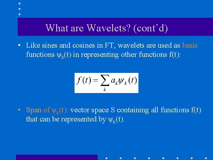
What are Wavelets? (cont’d) • Like sines and cosines in FT, wavelets are used as basis functions ψk(t) in representing other functions f(t): • Span of ψk(t): vector space S containing all functions f(t) that can be represented by ψk(t).

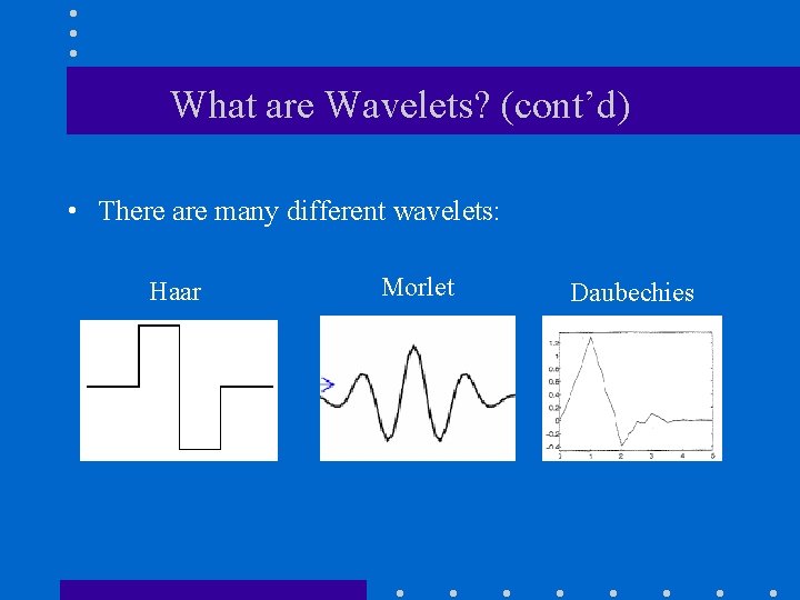
What are Wavelets? (cont’d) • There are many different wavelets: Haar Morlet Daubechies

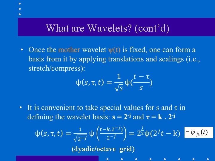
What are Wavelets? (cont’d) (dyadic/octave grid)

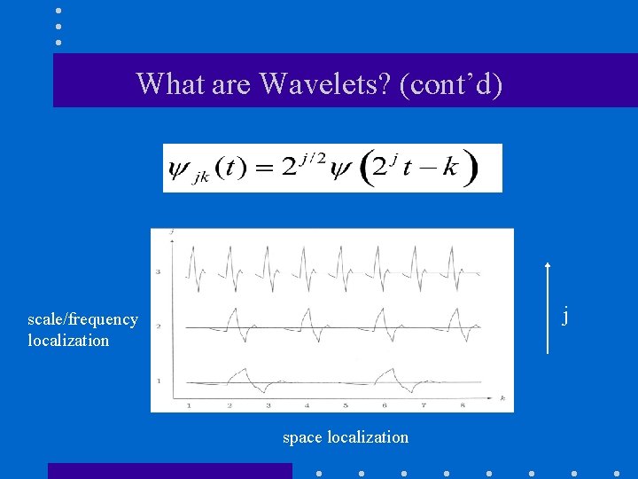
What are Wavelets? (cont’d) j scale/frequency localization space localization

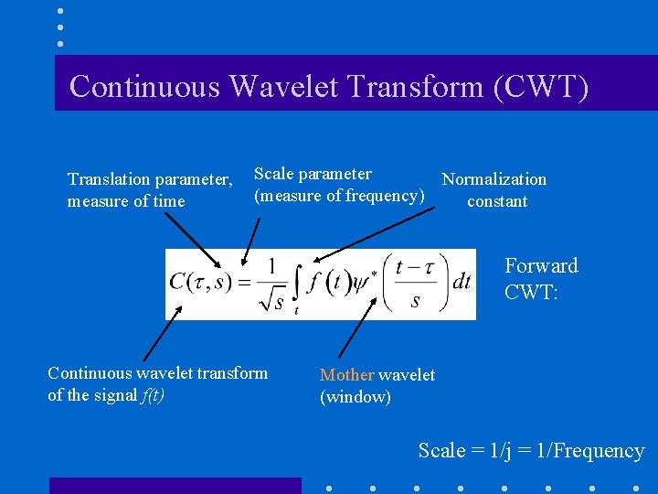
Continuous Wavelet Transform (CWT) Translation parameter, measure of time Scale parameter Normalization (measure of frequency) constant Forward CWT: Continuous wavelet transform of the signal f(t) Mother wavelet (window) Scale = 1/j = 1/Frequency

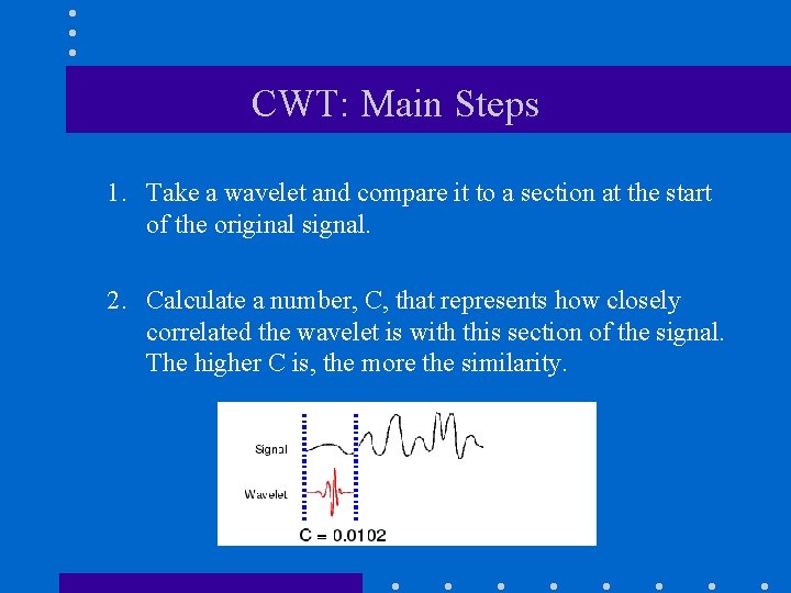
CWT: Main Steps 1. Take a wavelet and compare it to a section at the start of the original signal. 2. Calculate a number, C, that represents how closely correlated the wavelet is with this section of the signal. The higher C is, the more the similarity.

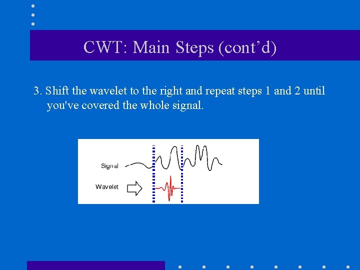
CWT: Main Steps (cont’d) 3. Shift the wavelet to the right and repeat steps 1 and 2 until you've covered the whole signal.

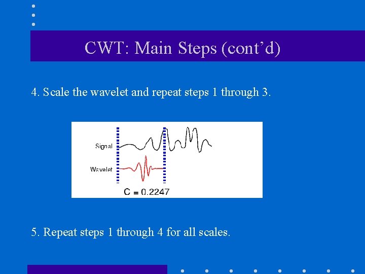
CWT: Main Steps (cont’d) 4. Scale the wavelet and repeat steps 1 through 3. 5. Repeat steps 1 through 4 for all scales.

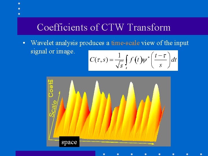
Coefficients of CTW Transform • Wavelet analysis produces a time-scale view of the input signal or image. space

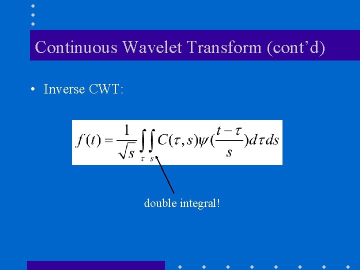
Continuous Wavelet Transform (cont’d) • Inverse CWT: double integral!

FT vs WT weighted by F(u) weighted by C(τ, s)

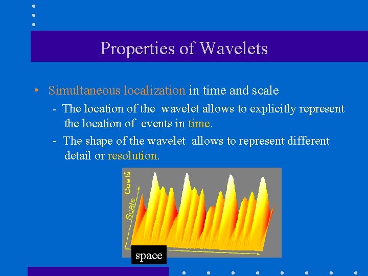
Properties of Wavelets • Simultaneous localization in time and scale - The location of the wavelet allows to explicitly represent the location of events in time. - The shape of the wavelet allows to represent different detail or resolution. space

Properties of Wavelets (cont’d) • Sparsity: for functions typically found in practice, many of the coefficients in a wavelet representation are either zero or very small. • Linear-time complexity: many wavelet transformations can be accomplished in O(N) time.

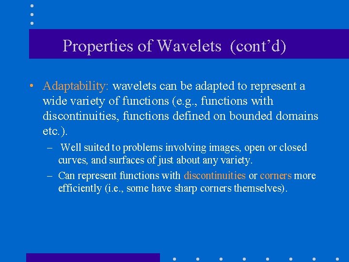
Properties of Wavelets (cont’d) • Adaptability: wavelets can be adapted to represent a wide variety of functions (e. g. , functions with discontinuities, functions defined on bounded domains etc. ). – Well suited to problems involving images, open or closed curves, and surfaces of just about any variety. – Can represent functions with discontinuities or corners more efficiently (i. e. , some have sharp corners themselves).

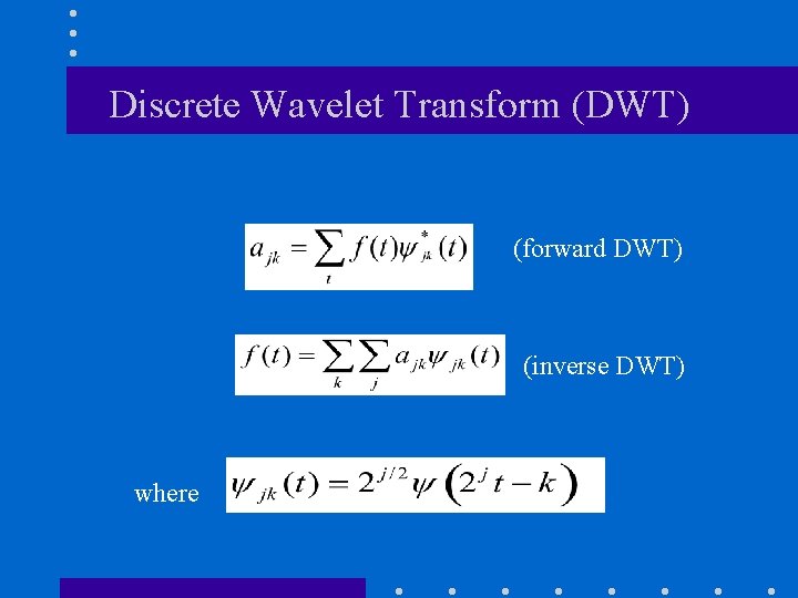
Discrete Wavelet Transform (DWT) (forward DWT) (inverse DWT) where

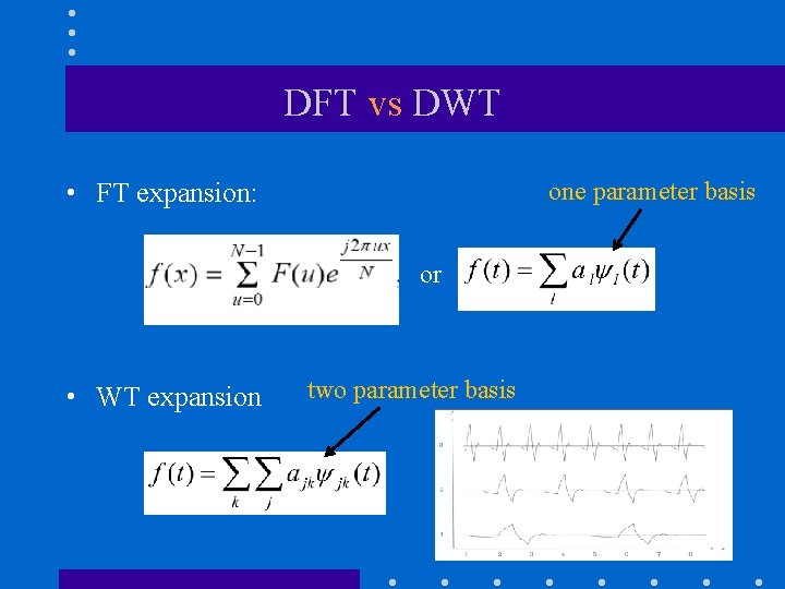
DFT vs DWT • FT expansion: one parameter basis or • WT expansion two parameter basis

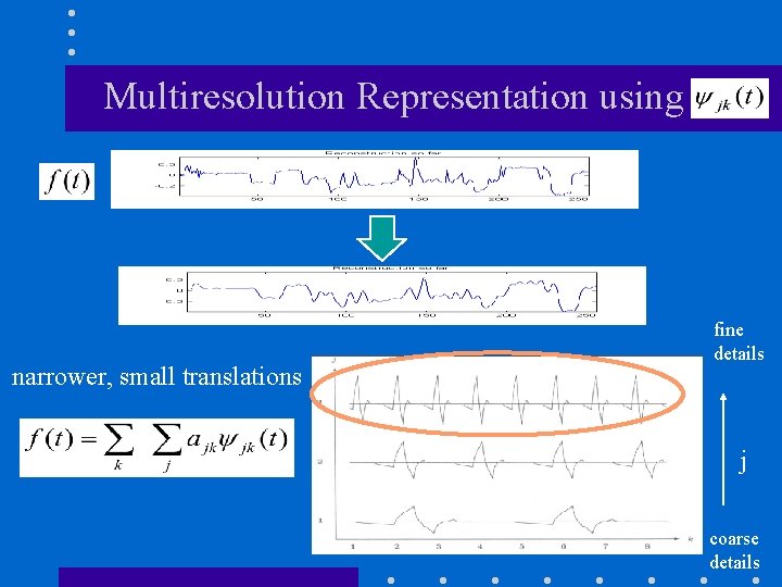
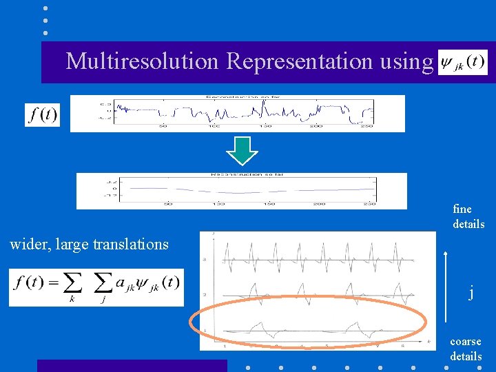
Multiresolution Representation using narrower, small translations fine details j coarse details

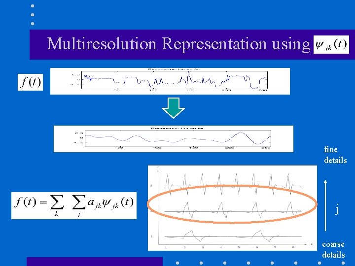
Multiresolution Representation using fine details j coarse details

Multiresolution Representation using fine details wider, large translations j coarse details

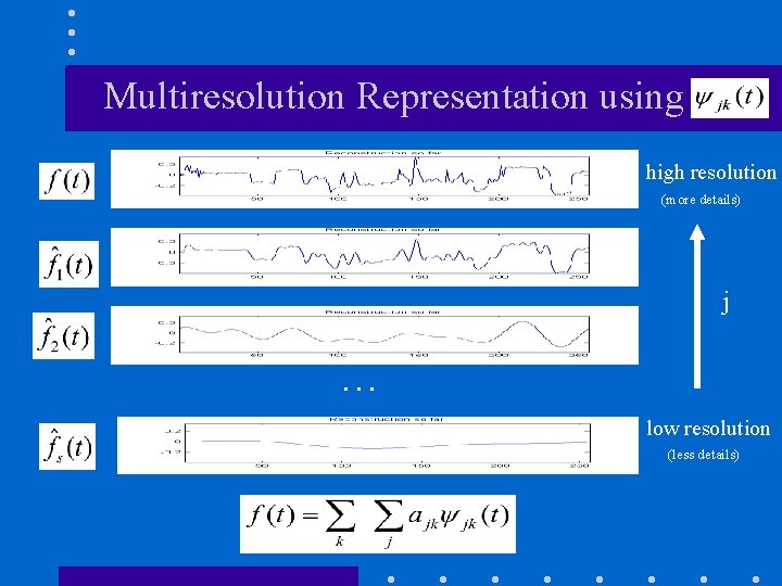
Multiresolution Representation using high resolution (more details) j … low resolution (less details)

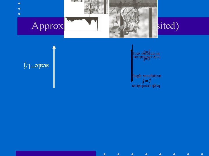
Approximation Pyramid (revisited) low resolution j=0 scale=1/j high resolution j=J

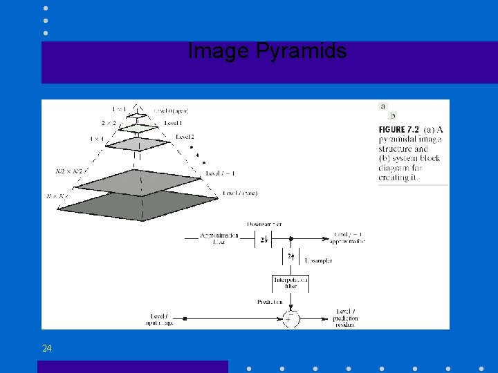
Image Pyramids 24

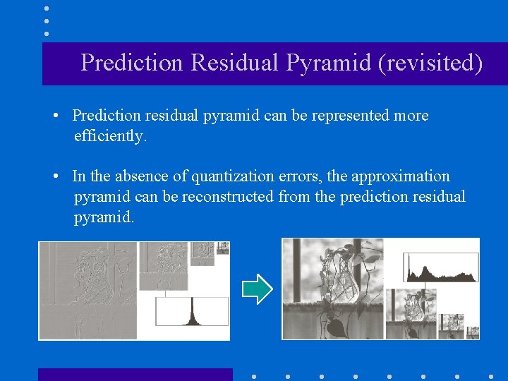
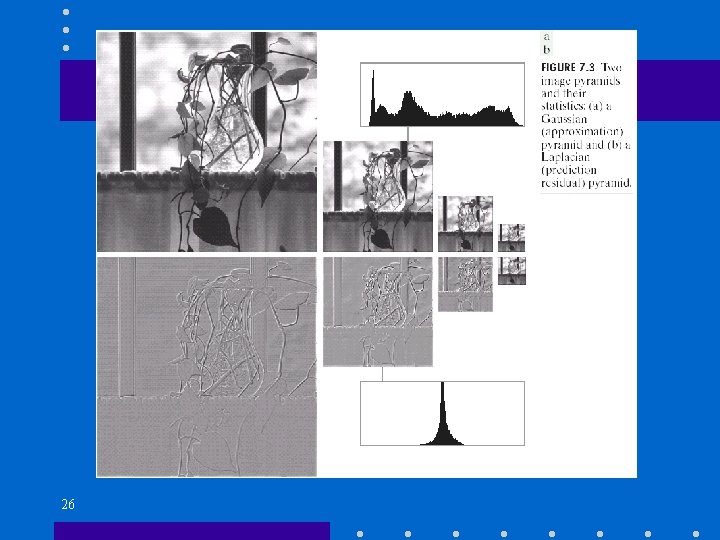
Prediction Residual Pyramid (revisited) • Prediction residual pyramid can be represented more efficiently. • In the absence of quantization errors, the approximation pyramid can be reconstructed from the prediction residual pyramid.

26

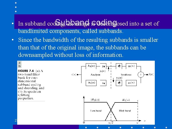
Subband coding • In subband coding, an image is decomposed into a set of bandlimited components, called subbands. • Since the bandwidth of the resulting subbands is smaller than that of the original image, the subbands can be downsampled without loss of information. 27

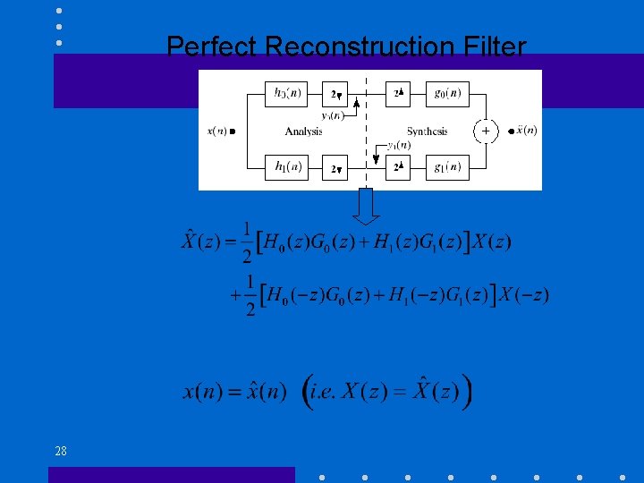
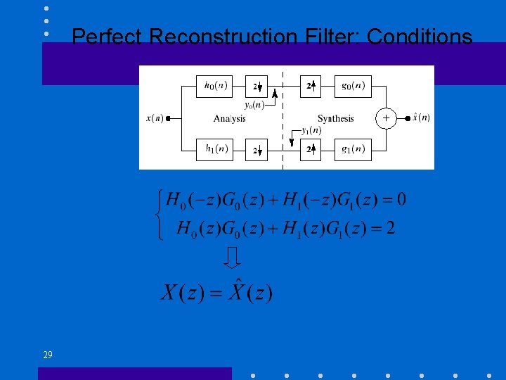
Perfect Reconstruction Filter Z transform: Goal: find H 0, H 1, G 0 and G 1 so that 28

Perfect Reconstruction Filter: Conditions If Then 29

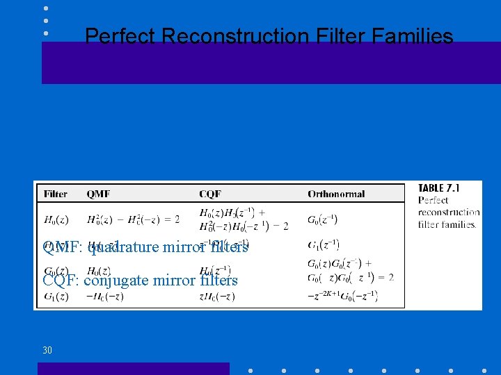
Perfect Reconstruction Filter Families QMF: quadrature mirror filters CQF: conjugate mirror filters 30

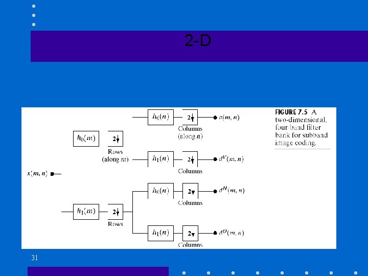
2 -D 31

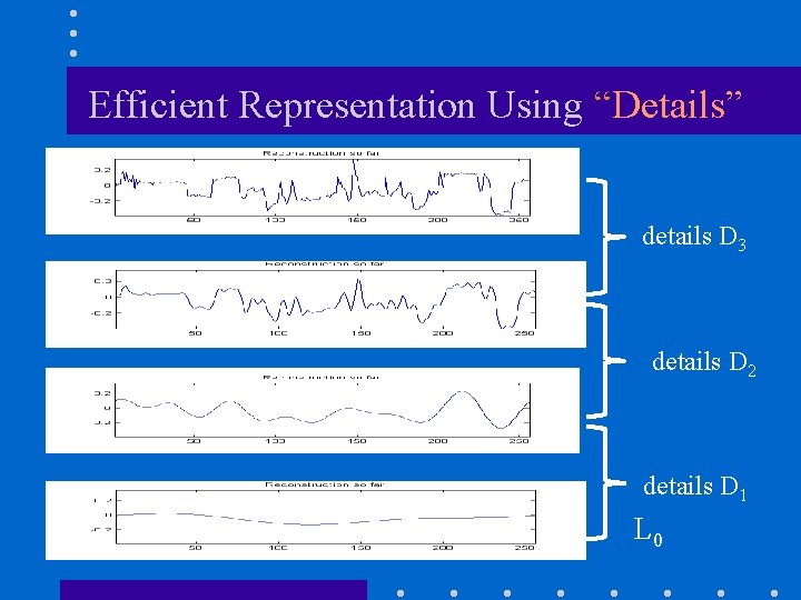
Efficient Representation Using “Details” details D 3 details D 2 details D 1 L 0

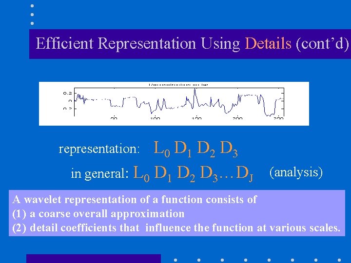
Efficient Representation Using Details (cont’d) L 0 D 1 D 2 D 3 in general: L 0 D 1 D 2 D 3…DJ representation: (analysis) A wavelet representation of a function consists of (1) a coarse overall approximation (2) detail coefficients that influence the function at various scales.

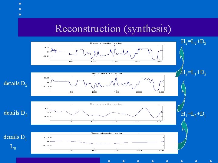
Reconstruction (synthesis) H 3=L 2+D 3 H 2=L 1+D 2 details D 3 details D 2 details D 1 L 0 H 1=L 0+D 1

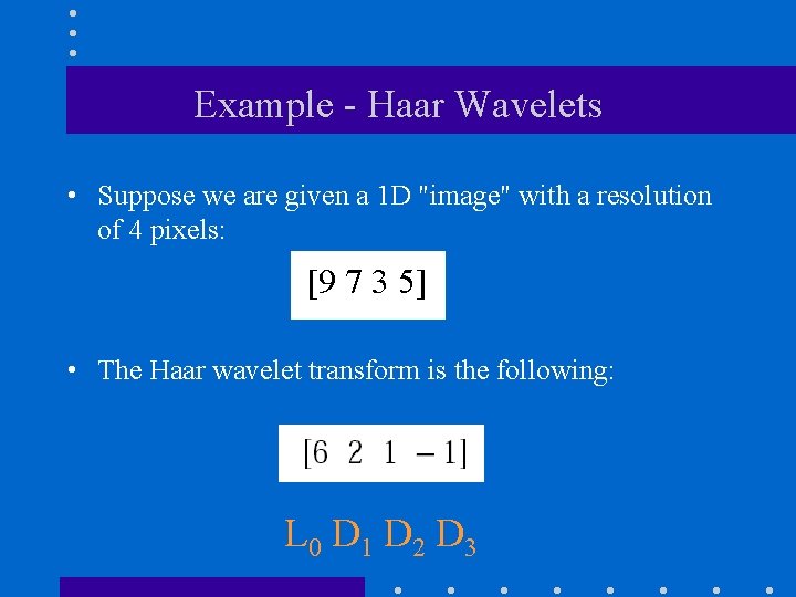
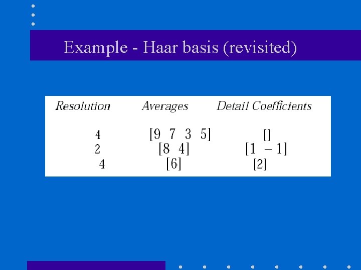
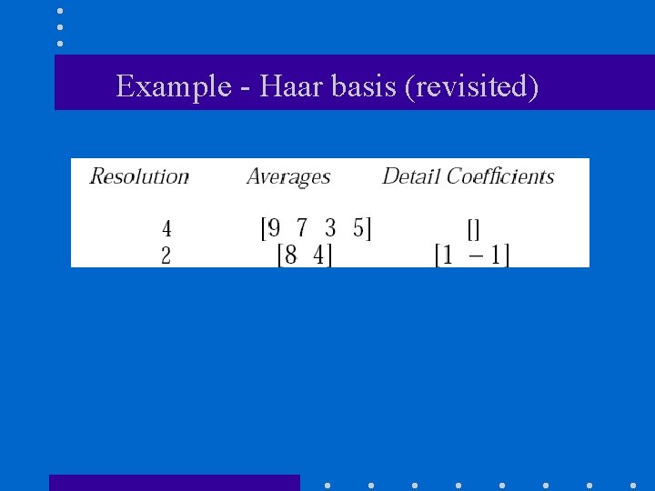
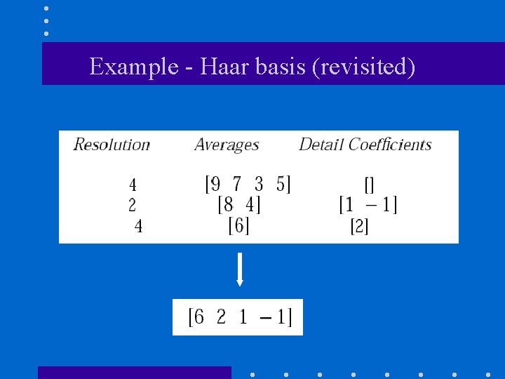
Example - Haar Wavelets • Suppose we are given a 1 D "image" with a resolution of 4 pixels: [9 7 3 5] • The Haar wavelet transform is the following: L 0 D 1 D 2 D 3

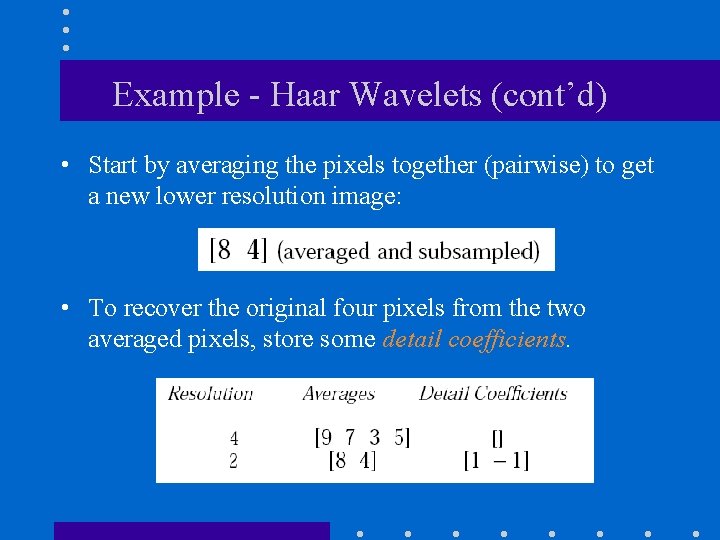
Example - Haar Wavelets (cont’d) • Start by averaging the pixels together (pairwise) to get a new lower resolution image: • To recover the original four pixels from the two averaged pixels, store some detail coefficients.

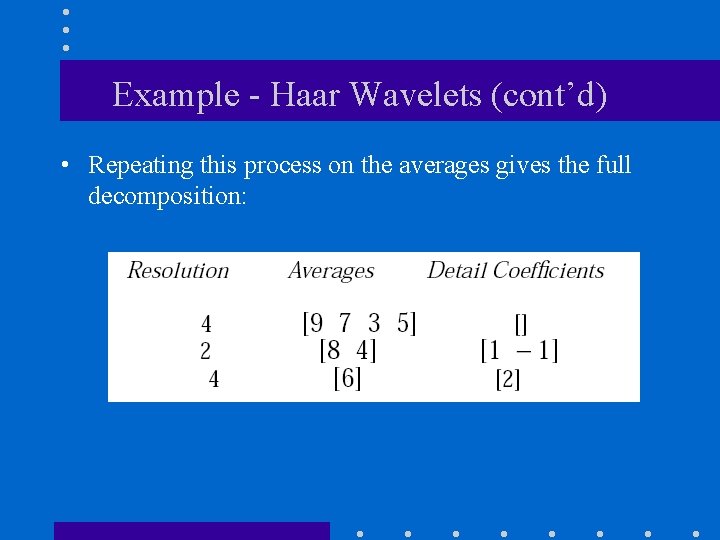
Example - Haar Wavelets (cont’d) • Repeating this process on the averages gives the full decomposition:

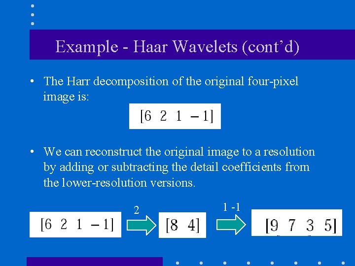
Example - Haar Wavelets (cont’d) • The Harr decomposition of the original four-pixel image is: • We can reconstruct the original image to a resolution by adding or subtracting the detail coefficients from the lower-resolution versions. 2 1 -1

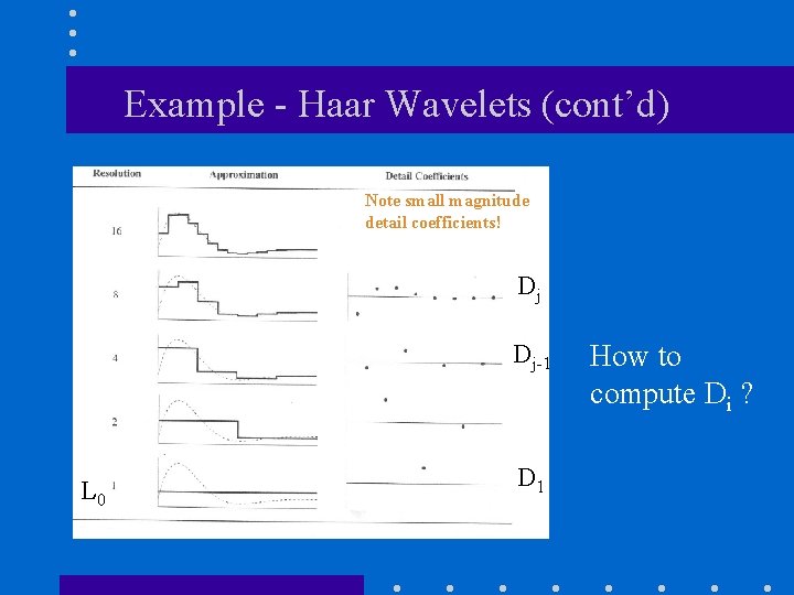
Example - Haar Wavelets (cont’d) Note small magnitude detail coefficients! Dj Dj-1 L 0 D 1 How to compute Di ?

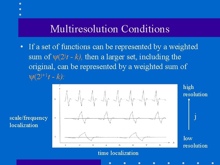
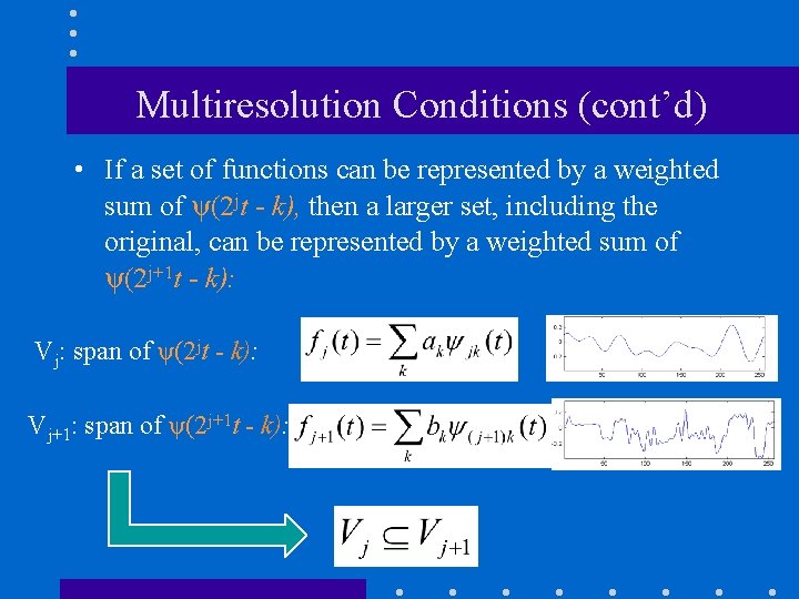
Multiresolution Conditions • If a set of functions can be represented by a weighted sum of ψ(2 jt - k), then a larger set, including the original, can be represented by a weighted sum of ψ(2 j+1 t - k): high resolution j scale/frequency localization low resolution time localization

Multiresolution Conditions (cont’d) • If a set of functions can be represented by a weighted sum of ψ(2 jt - k), then a larger set, including the original, can be represented by a weighted sum of ψ(2 j+1 t - k): Vj: span of ψ(2 jt - k): Vj+1: span of ψ(2 j+1 t - k):

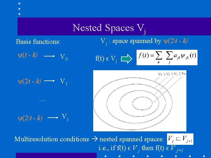
Nested Spaces Vj Vj : space spanned by ψ(2 jt - k) Basis functions: ψ(t - k) V 0 ψ(2 t - k) V 1 f(t) ϵ Vj … ψ(2 jt - k) Vj Multiresolution conditions nested spanned spaces: i. e. , if f(t) ϵ V j then f(t) ϵ V j+1

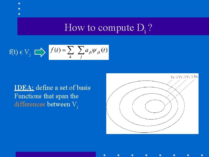
How to compute Di ? f(t) ϵ Vj IDEA: define a set of basis Functions that span the differences between Vj

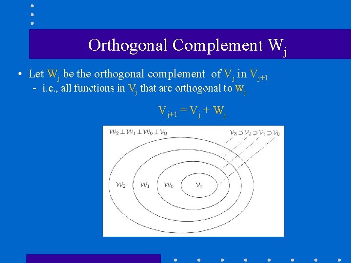
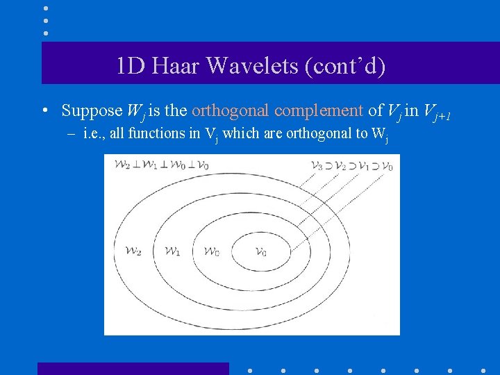
Orthogonal Complement Wj • Let Wj be the orthogonal complement of Vj in Vj+1 - i. e. , all functions in Vj that are orthogonal to Wj Vj+1 = Vj + Wj

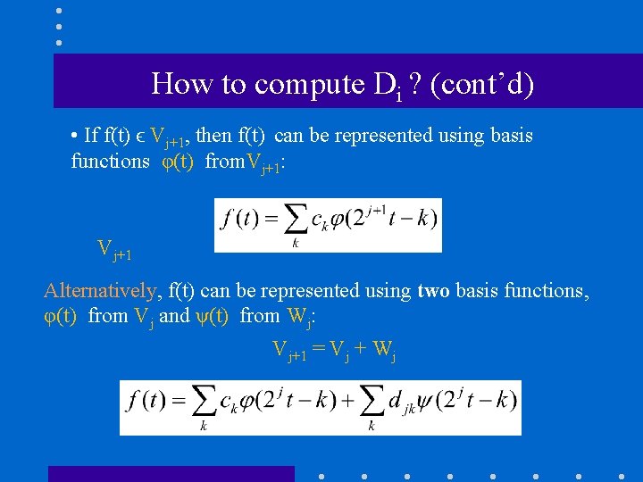
How to compute Di ? (cont’d) • If f(t) ϵ Vj+1, then f(t) can be represented using basis functions φ(t) from. Vj+1: Vj+1 Alternatively, f(t) can be represented using two basis functions, φ(t) from Vj and ψ(t) from Wj: Vj+1 = Vj + Wj

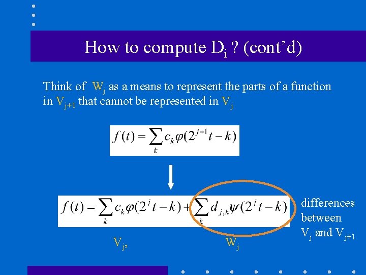
How to compute Di ? (cont’d) Think of Wj as a means to represent the parts of a function in Vj+1 that cannot be represented in Vj Vj , Wj differences between Vj and Vj+1

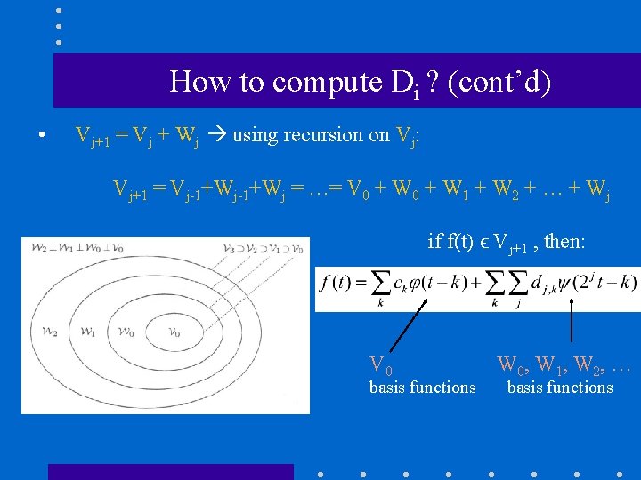
How to compute Di ? (cont’d) • Vj+1 = Vj + Wj using recursion on Vj: Vj+1 = Vj-1+Wj = …= V 0 + W 1 + W 2 + … + Wj if f(t) ϵ Vj+1 , then: V 0 basis functions W 0, W 1, W 2, … basis functions

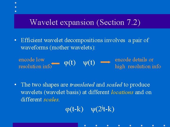
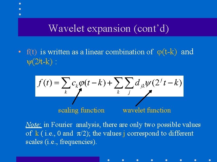
Wavelet expansion (Section 7. 2) • Efficient wavelet decompositions involves a pair of waveforms (mother wavelets): encode low resolution info φ(t) ψ(t) encode details or high resolution info • The two shapes are translated and scaled to produce wavelets (wavelet basis) at different locations and on different scales. φ(t-k) ψ(2 jt-k)

Wavelet expansion (cont’d) • f(t) is written as a linear combination of φ(t-k) and ψ(2 jt-k) : scaling function wavelet function Note: in Fourier analysis, there are only two possible values of k ( i. e. , 0 and π/2); the values j correspond to different scales (i. e. , frequencies).

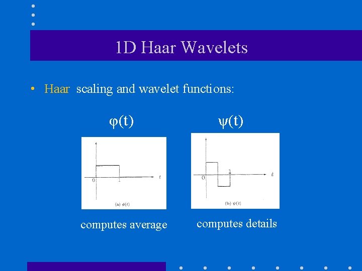
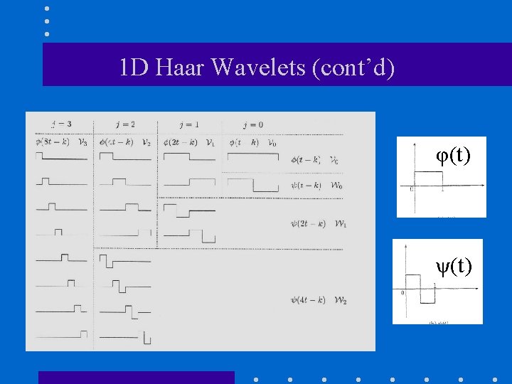
1 D Haar Wavelets • Haar scaling and wavelet functions: φ(t) computes average ψ(t) computes details

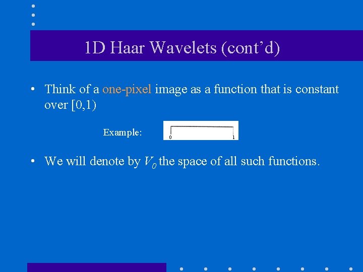
1 D Haar Wavelets (cont’d) • Think of a one-pixel image as a function that is constant over [0, 1) Example: 0 1 • We will denote by V 0 the space of all such functions.

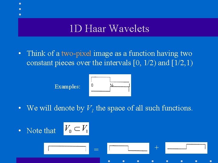
1 D Haar Wavelets • Think of a two-pixel image as a function having two constant pieces over the intervals [0, 1/2) and [1/2, 1) Examples: 0 ½ 1 • We will denote by V 1 the space of all such functions. • Note that = +

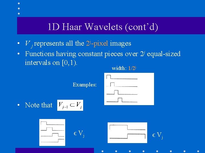
1 D Haar Wavelets (cont’d) • V j represents all the 2 j-pixel images • Functions having constant pieces over 2 j equal-sized intervals on [0, 1). j width: 1/2 Examples: • Note that ϵ Vj

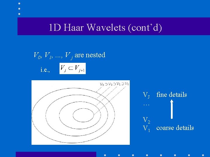
1 D Haar Wavelets (cont’d) V 0, V 1, . . . , V j are nested i. e. , VJ fine details … V 2 V 1 coarse details

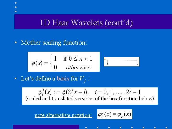
1 D Haar Wavelets (cont’d) • Mother scaling function: 1 0 • Let’s define a basis for V j : note alternative notation: 1

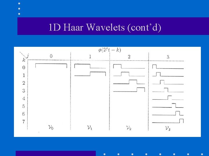
1 D Haar Wavelets (cont’d)

1 D Haar Wavelets (cont’d) • Suppose Wj is the orthogonal complement of Vj in Vj+1 – i. e. , all functions in Vj which are orthogonal to Wj

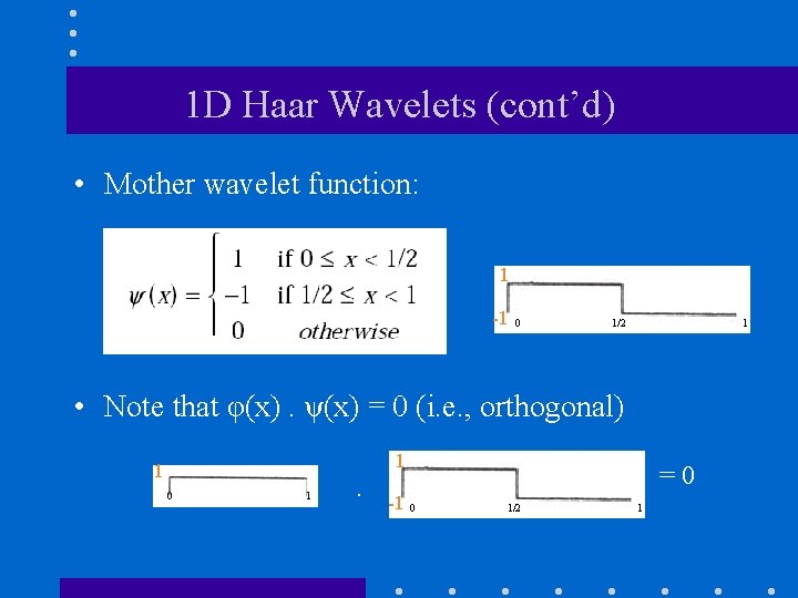
1 D Haar Wavelets (cont’d) • Mother wavelet function: 1 -1 0 1/2 1 • Note that φ(x). ψ(x) = 0 (i. e. , orthogonal) 1 1 0 1 . -1 =0 0 1/2 1

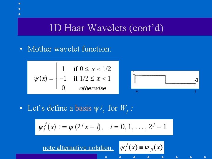
1 D Haar Wavelets (cont’d) • Mother wavelet function: 1 -1 0 • Let’s define a basis ψ ji for Wj : note alternative notation: 1

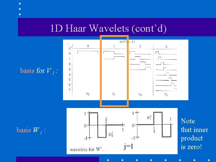
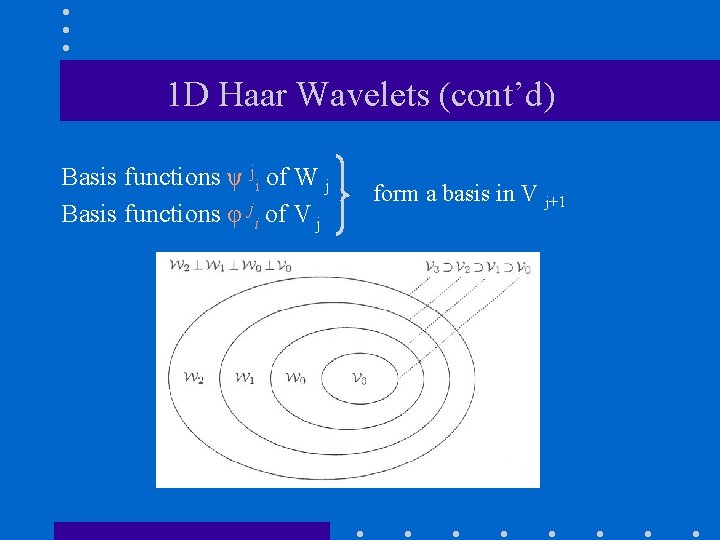
1 D Haar Wavelets (cont’d) basis for V 1 : basis W 1 : j=1 Note that inner product is zero!

1 D Haar Wavelets (cont’d) Basis functions ψ ji of W j Basis functions φ ji of V j form a basis in V j+1

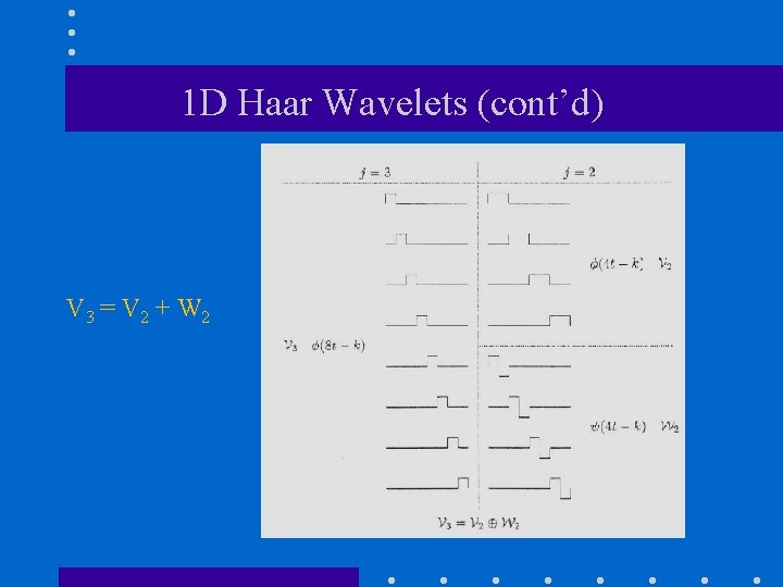
1 D Haar Wavelets (cont’d) V 3 = V 2 + W 2

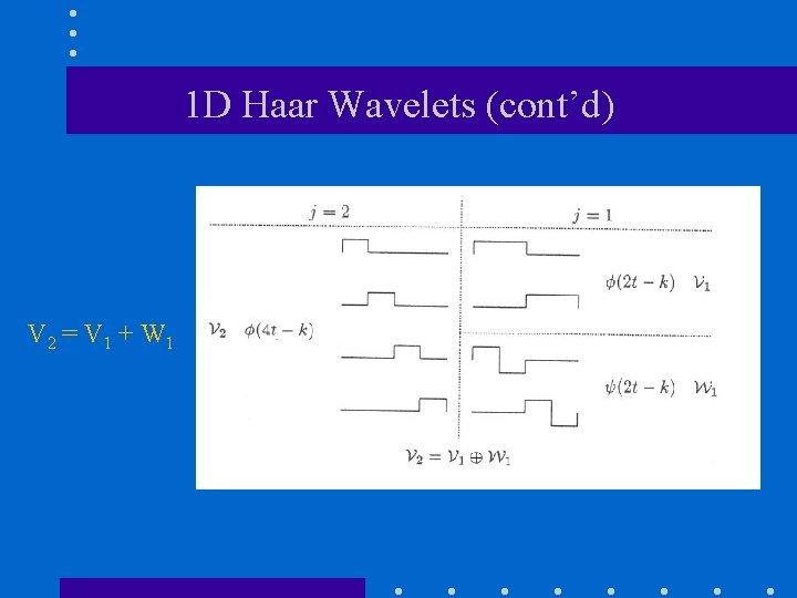
1 D Haar Wavelets (cont’d) V 2 = V 1 + W 1

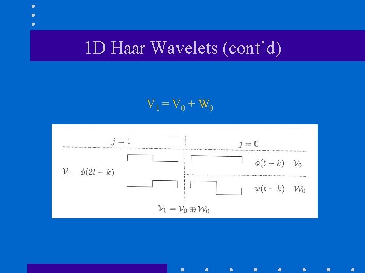
1 D Haar Wavelets (cont’d) V 1 = V 0 + W 0

1 D Haar Wavelets (cont’d) φ(t) ψ(t)

Example - Haar basis (revisited)

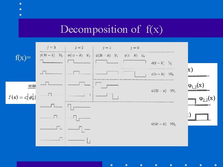
Decomposition of f(x)= φ0, 2(x) V 2 φ1, 2(x) φ2, 2(x) φ3, 2(x)

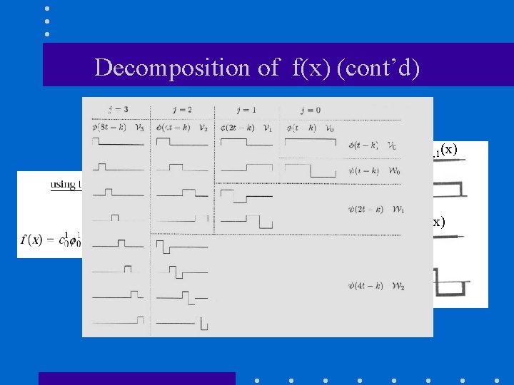
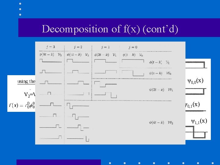
Decomposition of f(x) (cont’d) φ0, 1(x) V 1 and W 1 φ1, 1(x) V 2=V 1+W 1 ψ0, 1(x) ψ1, 1(x)

Example - Haar basis (revisited)

Decomposition of f(x) (cont’d) φ0, 0(x) V 0 , W 0 and W 1 ψ0, 0(x) V 2=V 1+W 1=V 0+W 1 ψ0, 1(x) ψ1, 1(x)

Example - Haar basis (revisited)

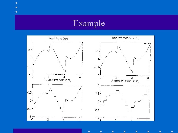
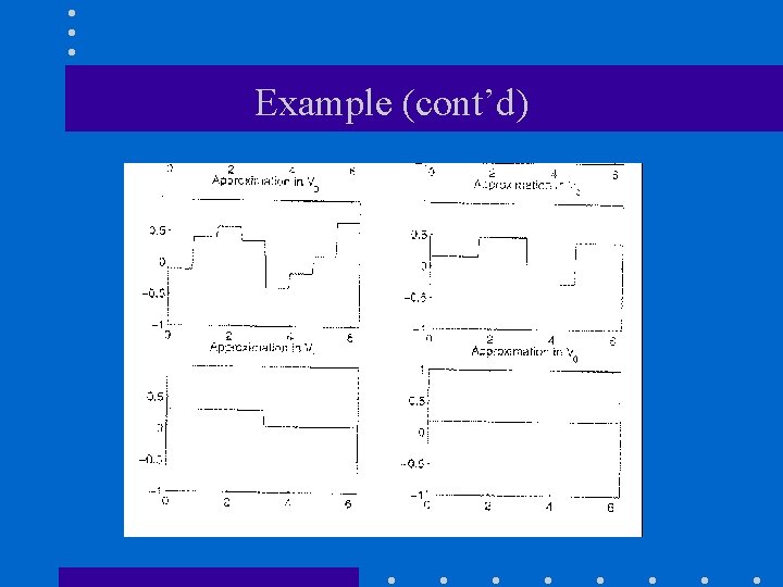
Example

Example (cont’d)

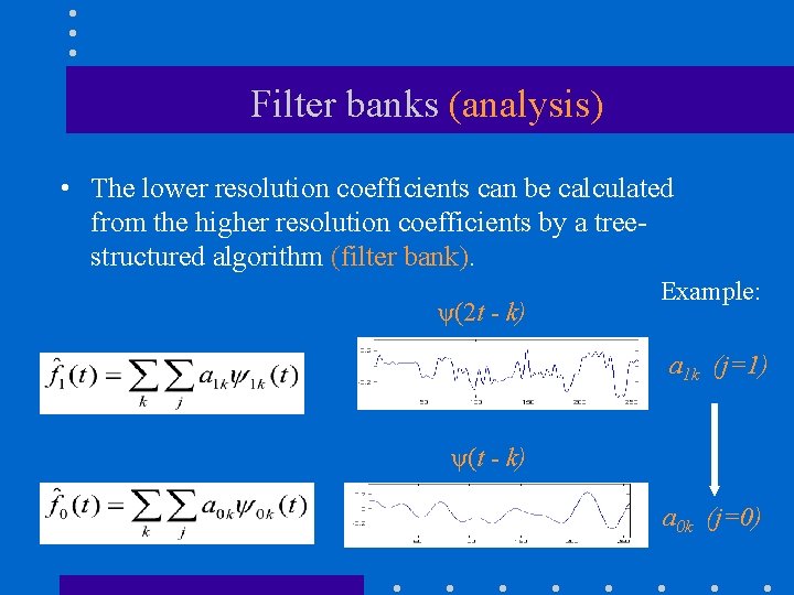
Filter banks (analysis) • The lower resolution coefficients can be calculated from the higher resolution coefficients by a treestructured algorithm (filter bank). ψ(2 t - k) Example: a 1 k (j=1) ψ(t - k) a 0 k (j=0)

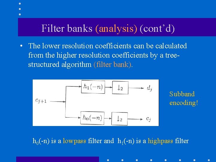
Filter banks (analysis) (cont’d) • The lower resolution coefficients can be calculated from the higher resolution coefficients by a treestructured algorithm (filter bank). Subband encoding! h 0(-n) is a lowpass filter and h 1(-n) is a highpass filter

Example - Haar basis (revisited) [9 7 3 5] low-pass, down-sampling (9+7)/2 high-pass, down-sampling (3+5)/2 (9 -7)/2 (3 -5)/2 V 1 basis functions

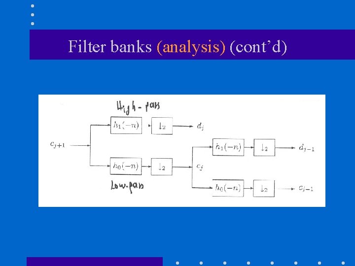
Filter banks (analysis) (cont’d)

Example - Haar basis (revisited) [9 7 3 5] low-pass, down-sampling high-pass, down-sampling V 1 basis functions (8+4)/2 (8 -4)/2

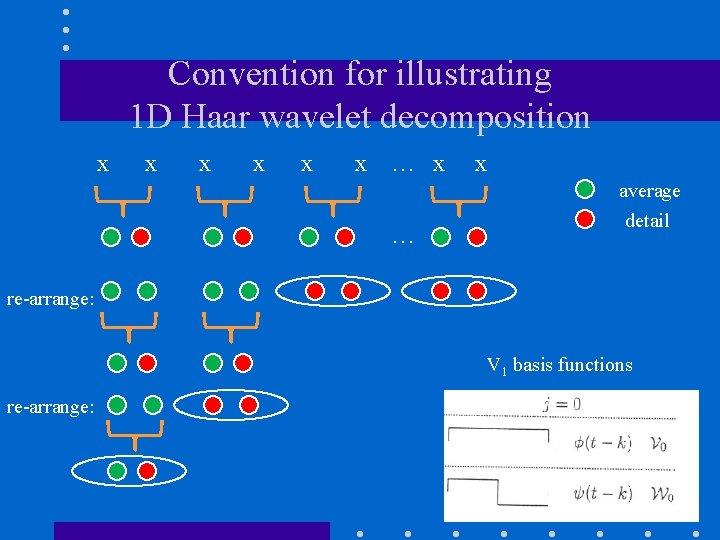
Convention for illustrating 1 D Haar wavelet decomposition x x x … x average detail re-arrange: V 1 basis functions re-arrange:

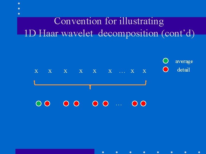
Convention for illustrating 1 D Haar wavelet decomposition (cont’d) x x x … x average detail

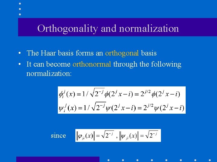
Orthogonality and normalization • The Haar basis forms an orthogonal basis • It can become orthonormal through the following normalization: since

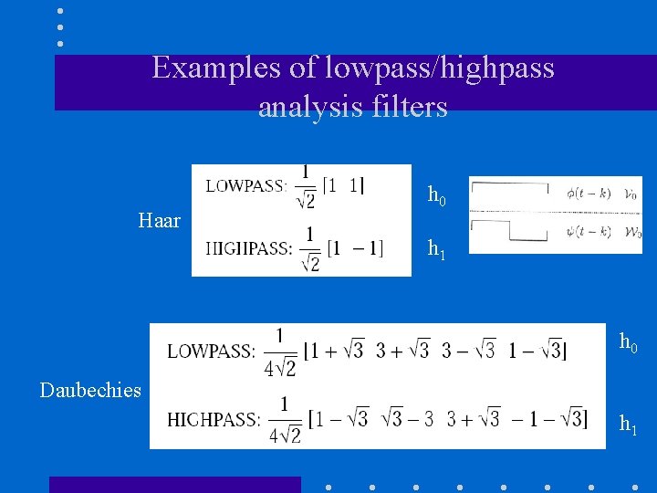
Examples of lowpass/highpass analysis filters Haar h 0 h 1 h 0 Daubechies h 1

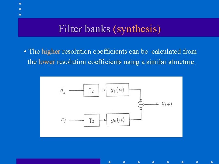
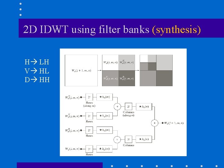
Filter banks (synthesis) • The higher resolution coefficients can be calculated from the lower resolution coefficients using a similar structure.

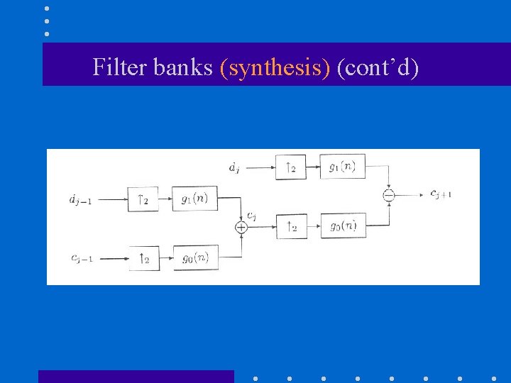
Filter banks (synthesis) (cont’d)

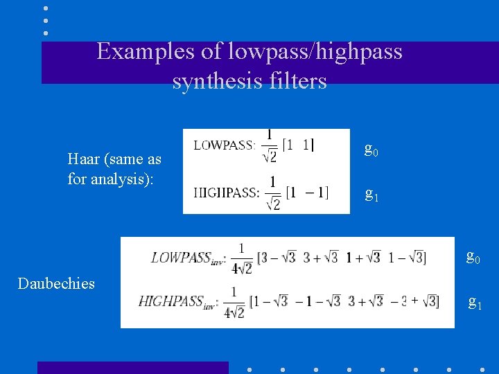
Examples of lowpass/highpass synthesis filters Haar (same as for analysis): g 0 g 1 g 0 Daubechies + g 1

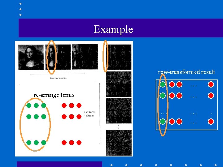
2 D Haar Wavelet Transform • The 2 D Haar wavelet decomposition can be computed using 1 D Haar wavelet decompositions (i. e. , 2 D Haar wavelet basis is separable). • Two decompositions – Standard decomposition – Non-standard decomposition • Each decomposition corresponds to a different set of 2 D basis functions.

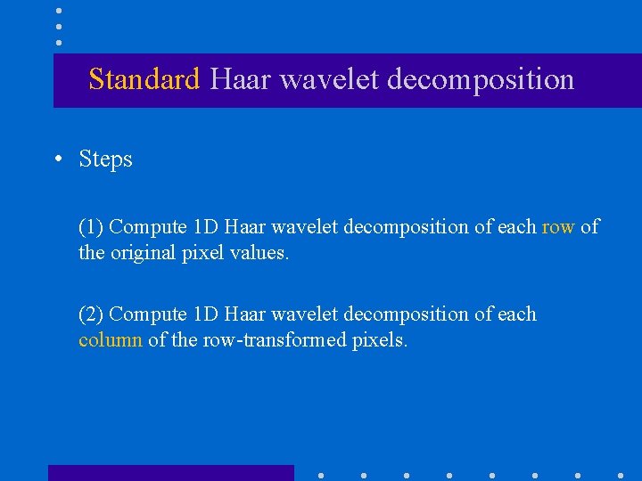
Standard Haar wavelet decomposition • Steps (1) Compute 1 D Haar wavelet decomposition of each row of the original pixel values. (2) Compute 1 D Haar wavelet decomposition of each column of the row-transformed pixels.

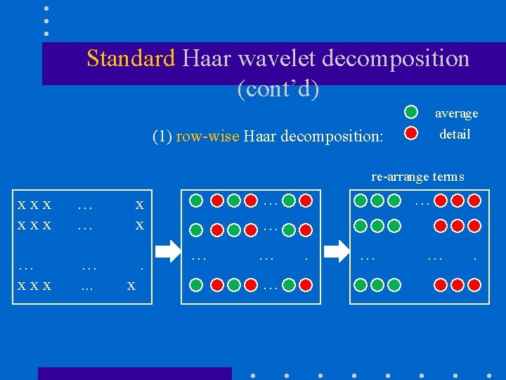
Standard Haar wavelet decomposition (cont’d) average detail (1) row-wise Haar decomposition: re-arrange terms xxx … … x x … xxx …. . x … … … .

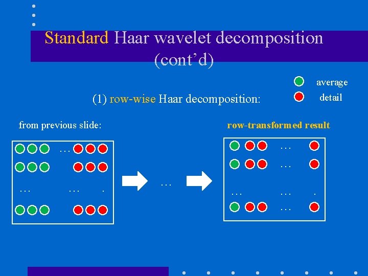
Standard Haar wavelet decomposition (cont’d) average detail (1) row-wise Haar decomposition: from previous slide: row-transformed result … … … .

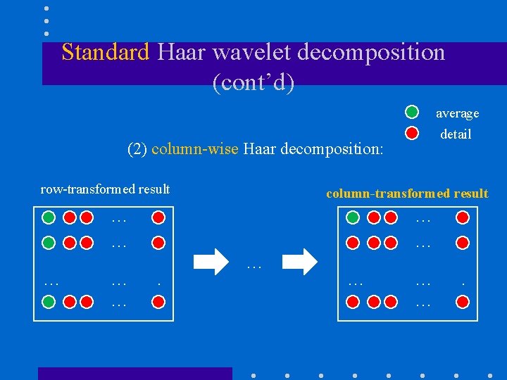
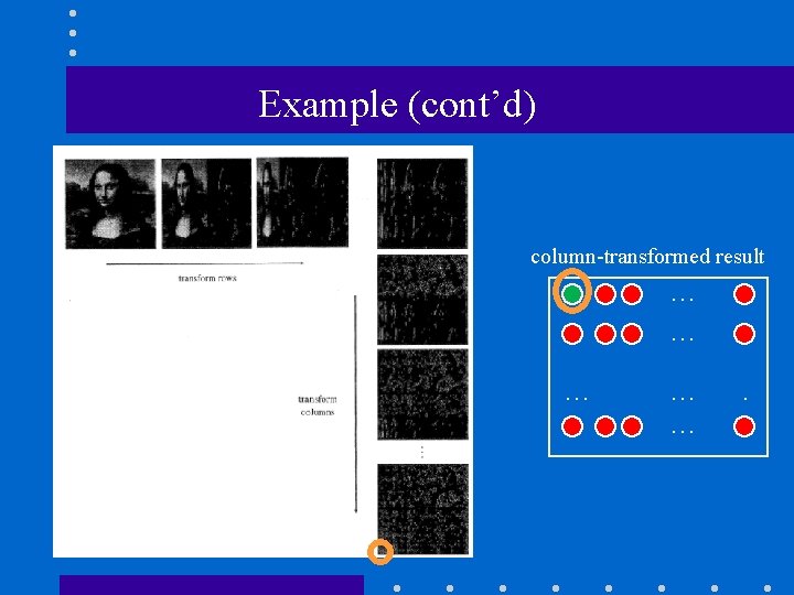
Standard Haar wavelet decomposition (cont’d) average detail (2) column-wise Haar decomposition: row-transformed result column-transformed result … … … … .

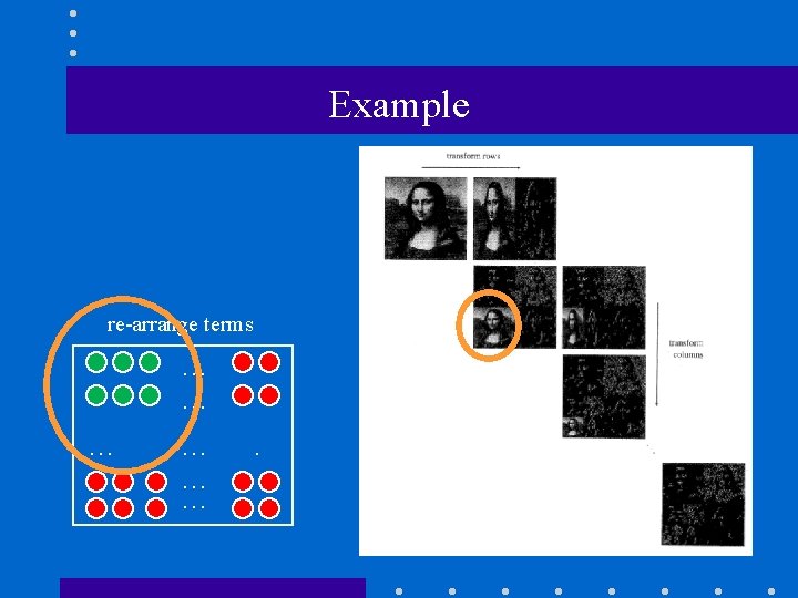
Example row-transformed result … … re-arrange terms … … .

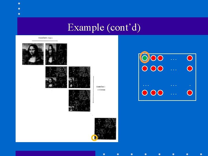
Example (cont’d) column-transformed result … … … .

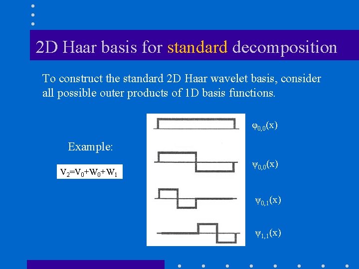
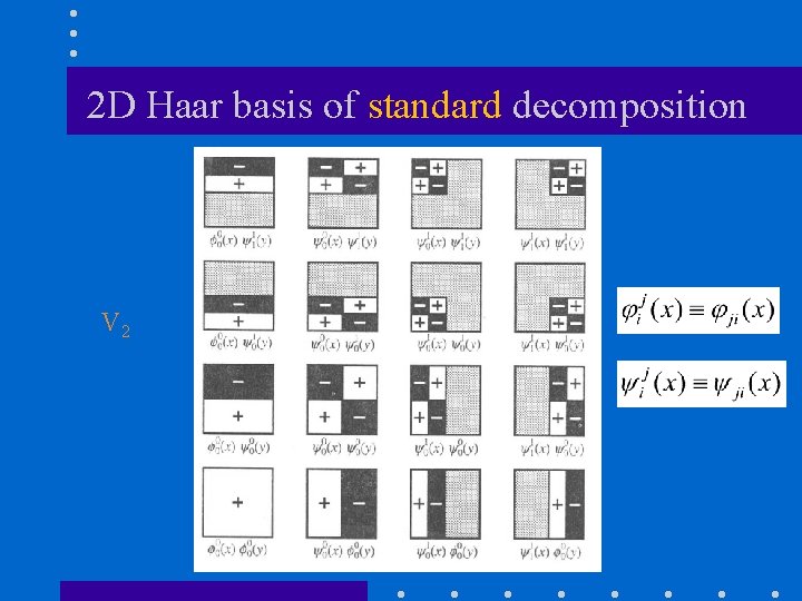
2 D Haar basis for standard decomposition To construct the standard 2 D Haar wavelet basis, consider all possible outer products of 1 D basis functions. φ0, 0(x) Example: V 2=V 0+W 1 ψ0, 0(x) ψ0, 1(x) ψ1, 1(x)

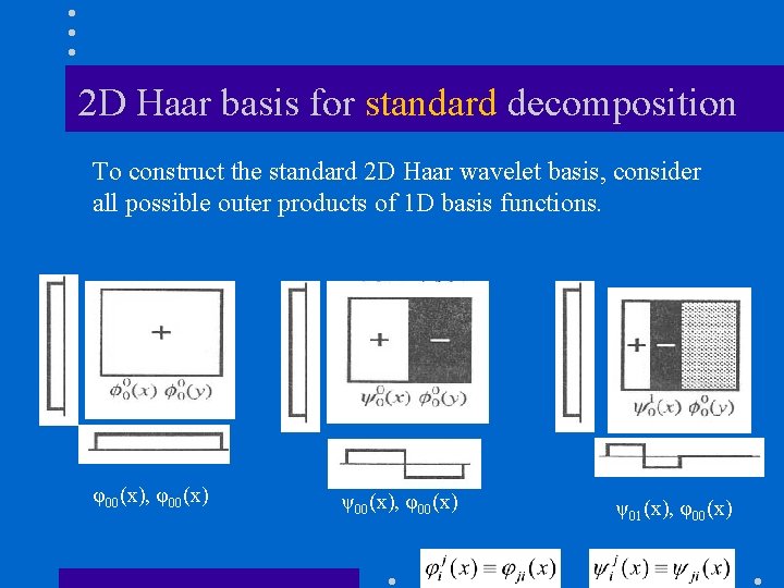
2 D Haar basis for standard decomposition To construct the standard 2 D Haar wavelet basis, consider all possible outer products of 1 D basis functions. φ00(x), φ00(x) ψ01(x), φ00(x)

2 D Haar basis of standard decomposition V 2

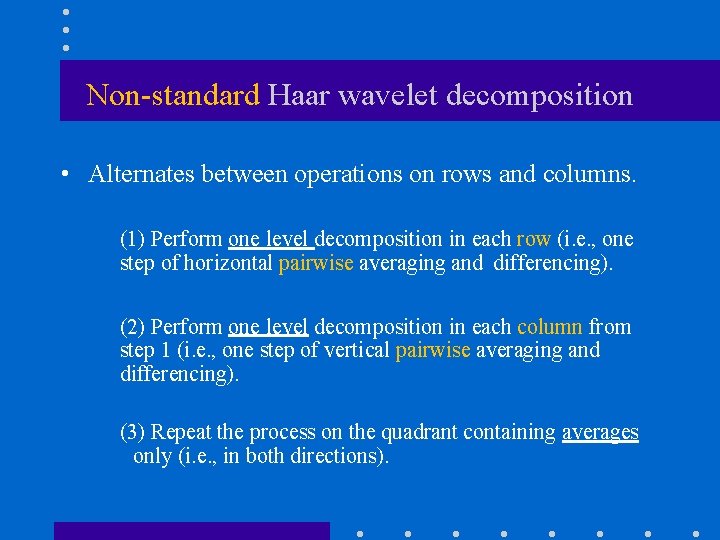
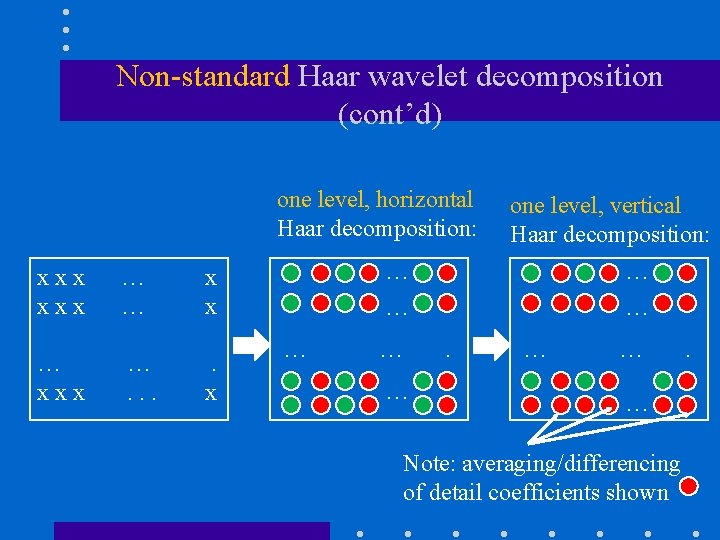
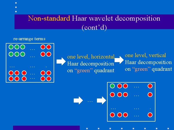
Non-standard Haar wavelet decomposition • Alternates between operations on rows and columns. (1) Perform one level decomposition in each row (i. e. , one step of horizontal pairwise averaging and differencing). (2) Perform one level decomposition in each column from step 1 (i. e. , one step of vertical pairwise averaging and differencing). (3) Repeat the process on the quadrant containing averages only (i. e. , in both directions).

Non-standard Haar wavelet decomposition (cont’d) one level, horizontal Haar decomposition: xxx … … x x … xxx …. . x one level, vertical Haar decomposition: … … … Note: averaging/differencing of detail coefficients shown .

Non-standard Haar wavelet decomposition (cont’d) re-arrange terms … … … . one level, horizontal Haar decomposition on “green” quadrant one level, vertical Haar decomposition on “green” quadrant … … … .

Example re-arrange terms … … … .

Example (cont’d) … … … .

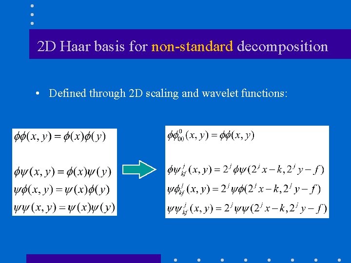
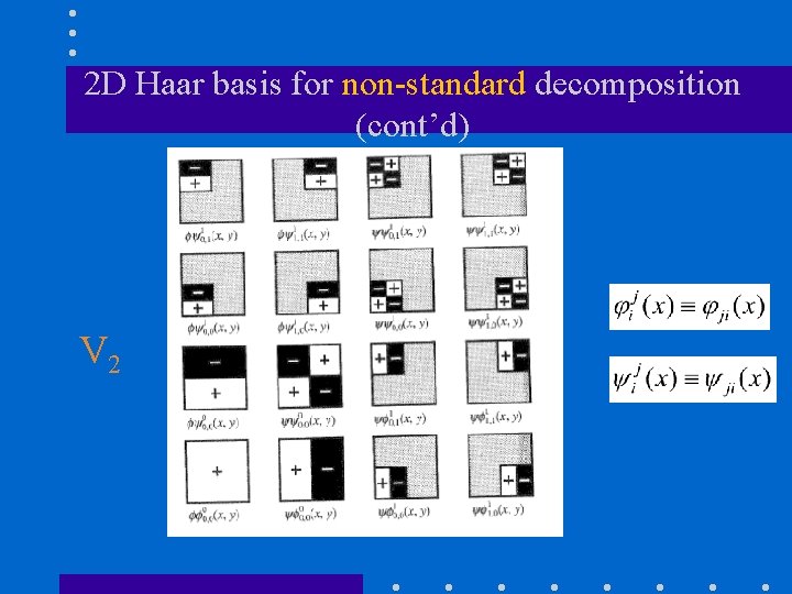
2 D Haar basis for non-standard decomposition • Defined through 2 D scaling and wavelet functions:

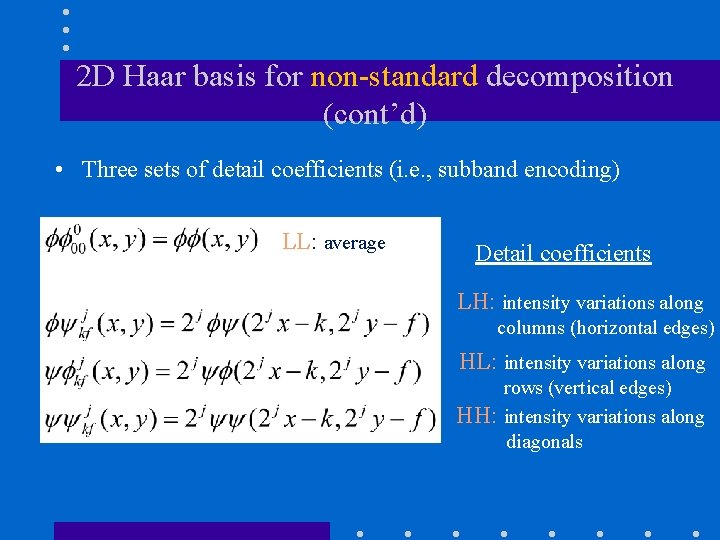
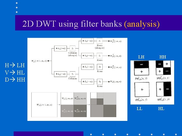
2 D Haar basis for non-standard decomposition (cont’d) • Three sets of detail coefficients (i. e. , subband encoding) LL: average LL Detail coefficients LH: intensity variations along columns (horizontal edges) HL: intensity variations along HH: rows (vertical edges) intensity variations along diagonals

2 D Haar basis for non-standard decomposition (cont’d) V 2

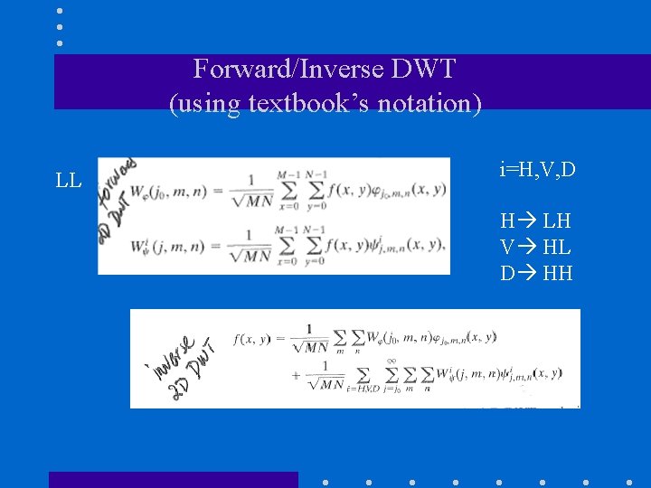
Forward/Inverse DWT (using textbook’s notation) LL i=H, V, D H LH V HL D HH

2 D DWT using filter banks (analysis) LH HH H LH V HL D HH LL HL

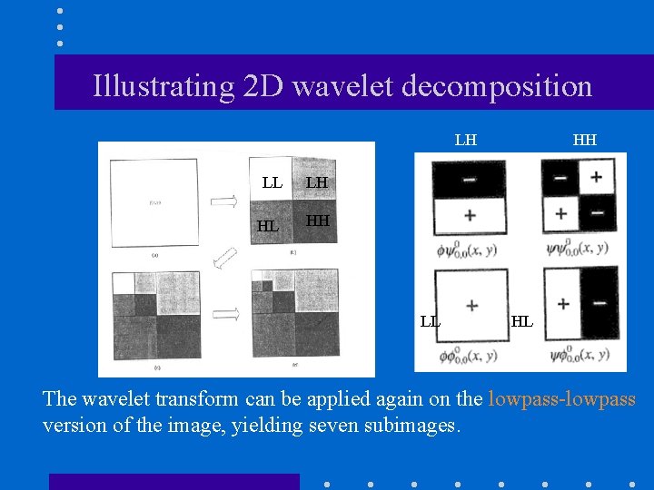
Illustrating 2 D wavelet decomposition LH LL LH HL HH LL HH HL The wavelet transform can be applied again on the lowpass-lowpass version of the image, yielding seven subimages.

2 D IDWT using filter banks (synthesis) H LH V HL D HH

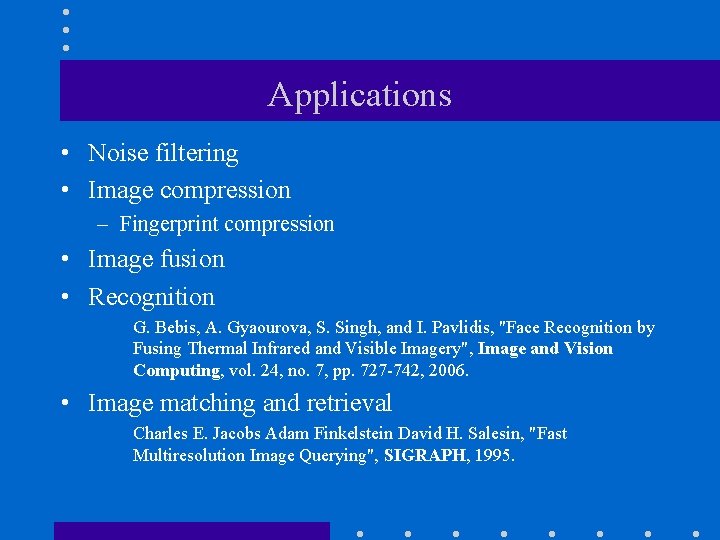
Applications • Noise filtering • Image compression – Fingerprint compression • Image fusion • Recognition G. Bebis, A. Gyaourova, S. Singh, and I. Pavlidis, "Face Recognition by Fusing Thermal Infrared and Visible Imagery", Image and Vision Computing, vol. 24, no. 7, pp. 727 -742, 2006. • Image matching and retrieval Charles E. Jacobs Adam Finkelstein David H. Salesin, "Fast Multiresolution Image Querying", SIGRAPH, 1995.

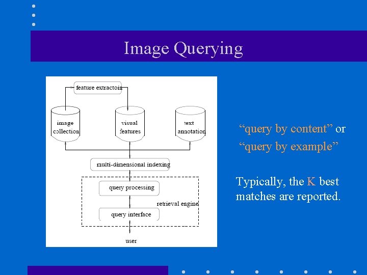
Image Querying “query by content” or “query by example” Typically, the K best matches are reported.

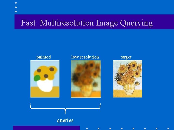
Fast Multiresolution Image Querying painted low resolution queries target