V 7 Digital pathology and MRI diagnostics Pathology

V 7 - Digital pathology and MRI diagnostics Pathology (from the Greek roots of pathos (πάθος), meaning "experience" or "suffering", and -logia (-λογία), "study of") is an important part of the causal study of diseases and a major field in modern medicine and diagnosis. Digital pathology (DP) includes all aspects of - acquisition, - process management, and - data interpretation to yield pathology information from a digitized pathology sample’s image. Program for today Q 1: Is the tissue healthy or cancer? Q 2: What cancer is it? Q 3: Where is the cancer? www. wikipedia. org Bhargava, Madabhushi Annu. Rev. Biomed. Eng. 2016. 18: 387– 412 V 7 WS 2018/19 Processing of Biological Data 1

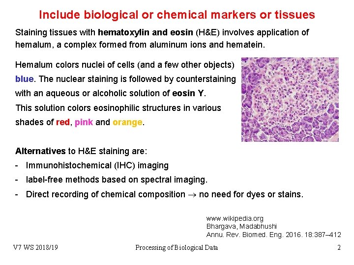
Include biological or chemical markers or tissues Staining tissues with hematoxylin and eosin (H&E) involves application of hemalum, a complex formed from aluminum ions and hematein. Hemalum colors nuclei of cells (and a few other objects) blue. The nuclear staining is followed by counterstaining with an aqueous or alcoholic solution of eosin Y. This solution colors eosinophilic structures in various shades of red, pink and orange. Alternatives to H&E staining are: - Immunohistochemical (IHC) imaging - label-free methods based on spectral imaging. - Direct recording of chemical composition no need for dyes or stains. www. wikipedia. org Bhargava, Madabhushi Annu. Rev. Biomed. Eng. 2016. 18: 387– 412 V 7 WS 2018/19 Processing of Biological Data 2

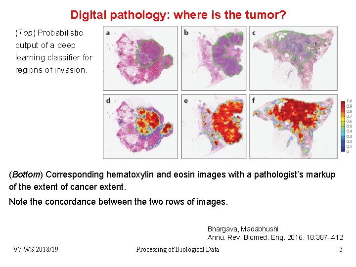
Digital pathology: where is the tumor? (Top) Probabilistic output of a deep learning classifier for regions of invasion. (Bottom) Corresponding hematoxylin and eosin images with a pathologist’s markup of the extent of cancer extent. Note the concordance between the two rows of images. Bhargava, Madabhushi Annu. Rev. Biomed. Eng. 2016. 18: 387– 412 V 7 WS 2018/19 Processing of Biological Data 3

Quantitative histomorphometry (QH) involves computerized image analysis tools for quantitatively assessing cancer tissue and non–cancer tissue morphology and architecture. QH measurements can be divided broadly into 3 groups: (a) architectural, (b) shape, and (c) texture based. V 7 WS 2018/19 Processing of Biological Data 4

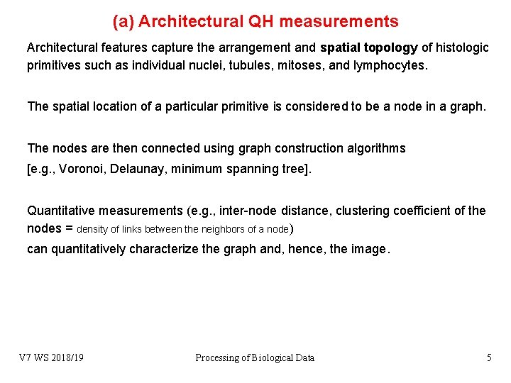
(a) Architectural QH measurements Architectural features capture the arrangement and spatial topology of histologic primitives such as individual nuclei, tubules, mitoses, and lymphocytes. The spatial location of a particular primitive is considered to be a node in a graph. The nodes are then connected using graph construction algorithms [e. g. , Voronoi, Delaunay, minimum spanning tree]. Quantitative measurements (e. g. , inter-node distance, clustering coefficient of the nodes = density of links between the neighbors of a node) can quantitatively characterize the graph and, hence, the image. V 7 WS 2018/19 Processing of Biological Data 5

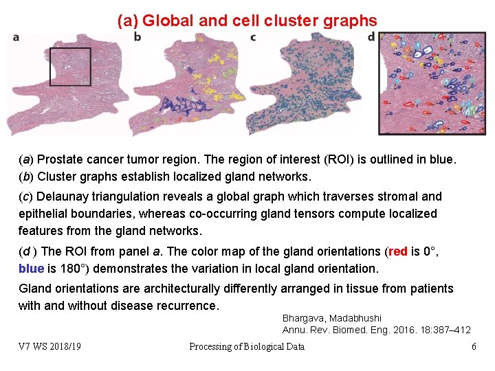
(a) Global and cell cluster graphs (a) Prostate cancer tumor region. The region of interest (ROI) is outlined in blue. (b) Cluster graphs establish localized gland networks. (c) Delaunay triangulation reveals a global graph which traverses stromal and epithelial boundaries, whereas co-occurring gland tensors compute localized features from the gland networks. (d ) The ROI from panel a. The color map of the gland orientations (red is 0°, blue is 180°) demonstrates the variation in local gland orientation. Gland orientations are architecturally differently arranged in tissue from patients with and without disease recurrence. Bhargava, Madabhushi Annu. Rev. Biomed. Eng. 2016. 18: 387– 412 V 7 WS 2018/19 Processing of Biological Data 6

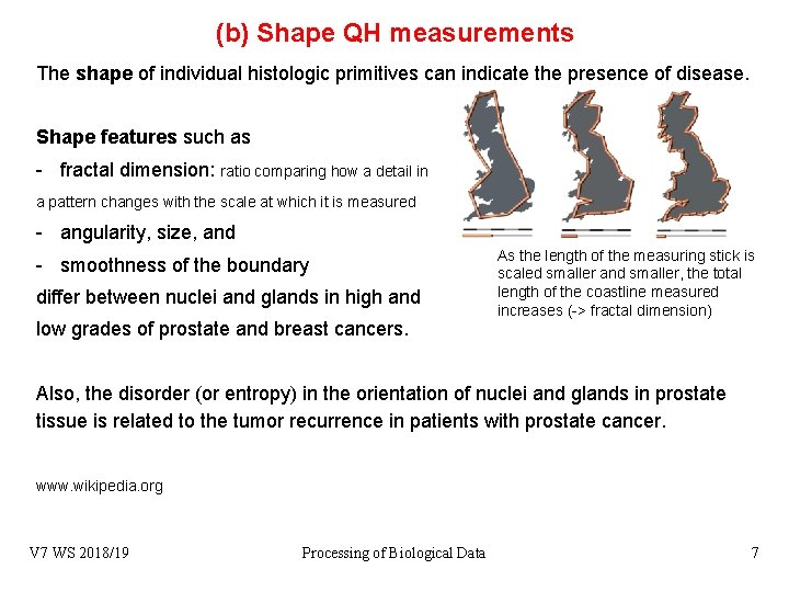
(b) Shape QH measurements The shape of individual histologic primitives can indicate the presence of disease. Shape features such as - fractal dimension: ratio comparing how a detail in a pattern changes with the scale at which it is measured - angularity, size, and - smoothness of the boundary differ between nuclei and glands in high and low grades of prostate and breast cancers. As the length of the measuring stick is scaled smaller and smaller, the total length of the coastline measured increases (-> fractal dimension) Also, the disorder (or entropy) in the orientation of nuclei and glands in prostate tissue is related to the tumor recurrence in patients with prostate cancer. www. wikipedia. org V 7 WS 2018/19 Processing of Biological Data 7

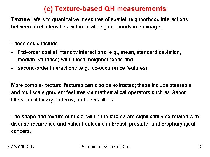
(c) Texture-based QH measurements Texture refers to quantitative measures of spatial neighborhood interactions between pixel intensities within local neighborhoods in an image. These could include - first-order spatial intensity interactions (e. g. , mean, standard deviation, median, variance) within local neighborhoods and - second-order interactions (e. g. , co-occurrence features). More complex textural features can also be extracted; these include steerable and multiscale gradient features via mathematical operators such as Gabor filters, local binary patterns, and Laws filters. The shape and texture of nuclei within the stroma are significantly correlated with disease recurrence and patient outcome in breast, prostate, and oropharyngeal cancers. V 7 WS 2018/19 Processing of Biological Data 8

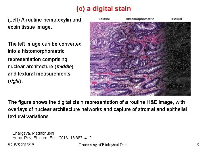
(c) a digital stain (Left) A routine hematoxylin and eosin tissue image. The left image can be converted into a histomorphometric representation comprising nuclear architecture (middle) and textural measurements (right). The figure shows the digital stain representation of a routine H&E image, with overlays of nuclear architecture networks and capture of stromal and epithelial textural variations. Bhargava, Madabhushi Annu. Rev. Biomed. Eng. 2016. 18: 387– 412 V 7 WS 2018/19 Processing of Biological Data 9

Principles of chemical imaging IR imaging provides high image contrast, fast data recording, and high molecular sensitivity. Vibrational frequencies within molecules directly resonate with optical frequencies in the mid-IR spectral region. Thus, light absorption provides a quantitative molecular fingerprint of the material, providing ample molecular biomarkers. No dyes or stains are needed to visualize molecular content. Data can be recorded without prior knowledge of the type or composition of the sample. V 7 WS 2018/19 Processing of Biological Data 10

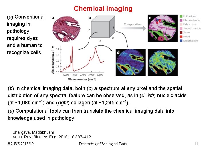
Chemical imaging (a) Conventional imaging in pathology requires dyes and a human to recognize cells. (b) In chemical imaging data, both (c) a spectrum at any pixel and the spatial distribution of any spectral feature can be observed, as in (d, left) nucleic acids (at ∼ 1, 080 cm− 1) and (right) collagen (at ∼ 1, 245 cm− 1). (e) Computational tools can then translate the chemical imaging data into knowledge used in pathology. Bhargava, Madabhushi Annu. Rev. Biomed. Eng. 2016. 18: 387– 412 V 7 WS 2018/19 Processing of Biological Data 11

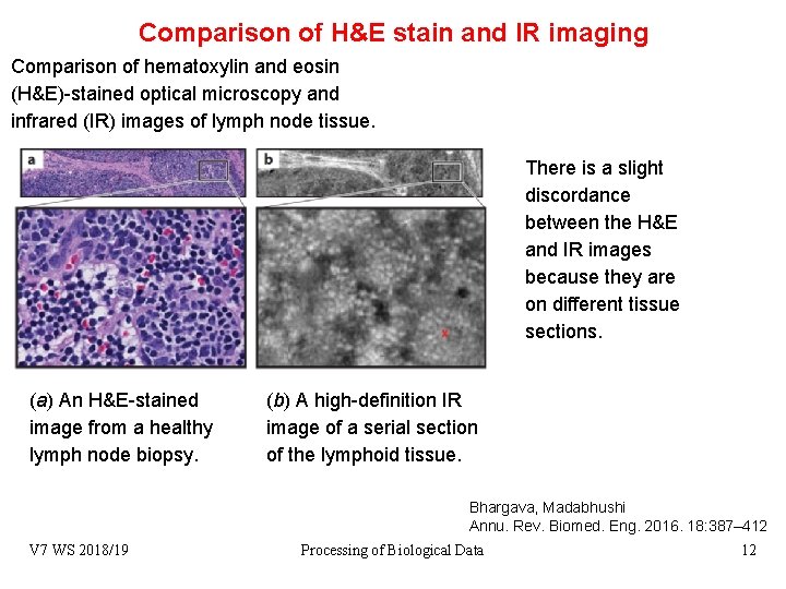
Comparison of H&E stain and IR imaging Comparison of hematoxylin and eosin (H&E)-stained optical microscopy and infrared (IR) images of lymph node tissue. There is a slight discordance between the H&E and IR images because they are on different tissue sections. (a) An H&E-stained image from a healthy lymph node biopsy. (b) A high-definition IR image of a serial section of the lymphoid tissue. Bhargava, Madabhushi Annu. Rev. Biomed. Eng. 2016. 18: 387– 412 V 7 WS 2018/19 Processing of Biological Data 12

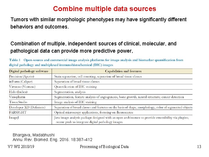
Combine multiple data sources Tumors with similar morphologic phenotypes may have significantly different behaviors and outcomes. Combination of multiple, independent sources of clinical, molecular, and pathological data can provide more predictive power, Bhargava, Madabhushi Annu. Rev. Biomed. Eng. 2016. 18: 387– 412 V 7 WS 2018/19 Processing of Biological Data 13

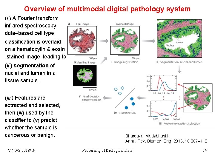
Overview of multimodal digital pathology system (i ) A Fourier transform infrared spectroscopy data–based cell type classification is overlaid on a hematoxylin & eosin -stained image, leading to (ii ) segmentation of nuclei and lumen in a tissue sample. (iii ) Features are extracted and selected, then (iv) used by the classifier to (v) predict whether the sample is cancerous or benign. V 7 WS 2018/19 Bhargava, Madabhushi Annu. Rev. Biomed. Eng. 2016. 18: 387– 412 Processing of Biological Data 14

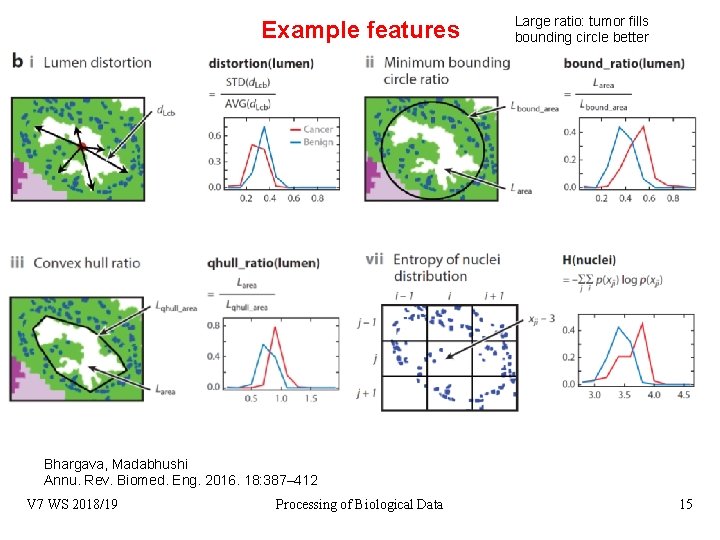
Example features Large ratio: tumor fills bounding circle better Bhargava, Madabhushi Annu. Rev. Biomed. Eng. 2016. 18: 387– 412 V 7 WS 2018/19 Processing of Biological Data 15

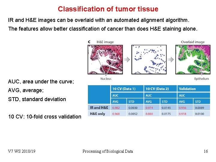
Classification of tumor tissue IR and H&E images can be overlaid with an automated alignment algorithm. The features allow better classification of cancer than does H&E staining alone. AUC, area under the curve; AVG, average; STD, standard deviation 10 CV: 10 -fold cross validation V 7 WS 2018/19 Processing of Biological Data 16

Analysis of digitized images A typical analysis pipeline involves a machine learning classifier that takes as input a series of manually or computer-extracted features and employs those features to render a prediction. In the context of digital pathology, predictions might involve - a low-level recognition (e. g. , Is the primitive a nucleus or not? ), - a diagnostic decision (e. g. , Is the tissue region of interest cancerous or not? ), - or a prognostication (e. g. , Will the patient have early or distant disease recurrence? ). V 7 WS 2018/19 Processing of Biological Data 17

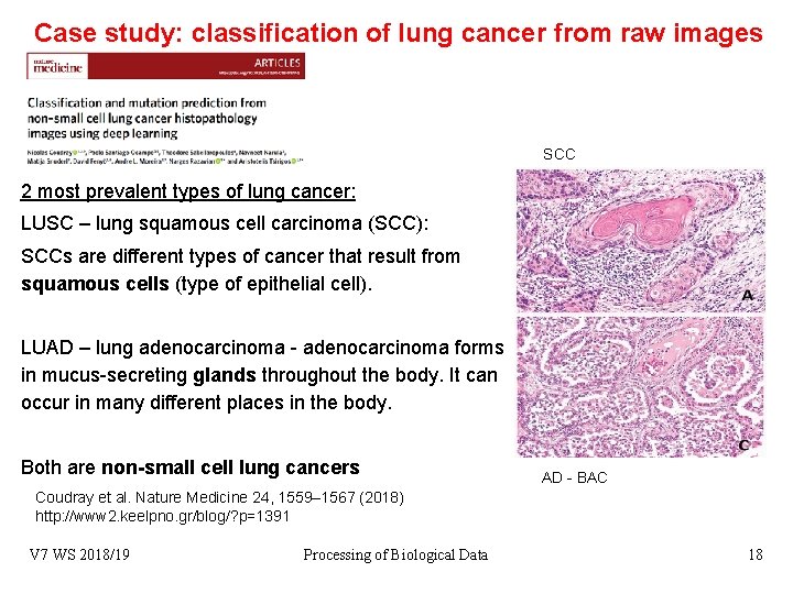
Case study: classification of lung cancer from raw images SCC 2 most prevalent types of lung cancer: LUSC – lung squamous cell carcinoma (SCC): SCCs are different types of cancer that result from squamous cells (type of epithelial cell). LUAD – lung adenocarcinoma - adenocarcinoma forms in mucus-secreting glands throughout the body. It can occur in many different places in the body. Both are non-small cell lung cancers AD - BAC Coudray et al. Nature Medicine 24, 1559– 1567 (2018) http: //www 2. keelpno. gr/blog/? p=1391 V 7 WS 2018/19 Processing of Biological Data 18

Treatment of LUAC / LUSC Stage I – surgery or radiation therapy Stage II – surgery and chemotherapy or radiation therapy Stage III – sequential or concurrent chemotherapy and radiation therapy, more options … Stage IV – patient genetics becomes important - Cytotoxic combination chemotherapy - Combination chemotherapy with monoclonal antibodies - Maintenance therapy after first-line chemotherapy (for patients with stable or responding disease after 4 cycles of platinum-based combination chemotherapy) - EGFR tyrosine kinase inhibitors - ALK inhibitors (for patients with ALK translocations) - ROS 1 inhibitors (for patients with ROS 1 rearrangements) - BRAFV 600 E and MEK inhibitors (for patients with BRAFV 600 E mutations) - Immune checkpoint inhibitors with or without chemotherapy https: //www. cancer. gov/types/lung/hp/non-small-cell-lung-treatment-pdq#section/_48406 V 7 WS 2018/19 Processing of Biological Data 19

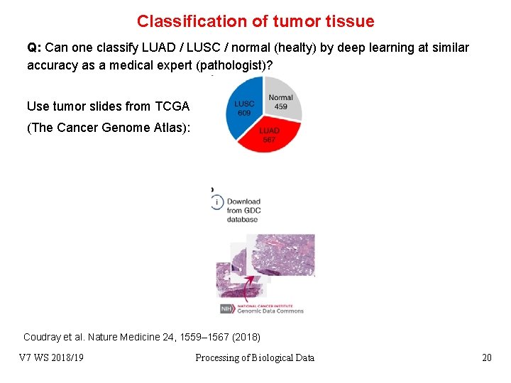
Classification of tumor tissue Q: Can one classify LUAD / LUSC / normal (healty) by deep learning at similar accuracy as a medical expert (pathologist)? Use tumor slides from TCGA (The Cancer Genome Atlas): Coudray et al. Nature Medicine 24, 1559– 1567 (2018) V 7 WS 2018/19 Processing of Biological Data 20

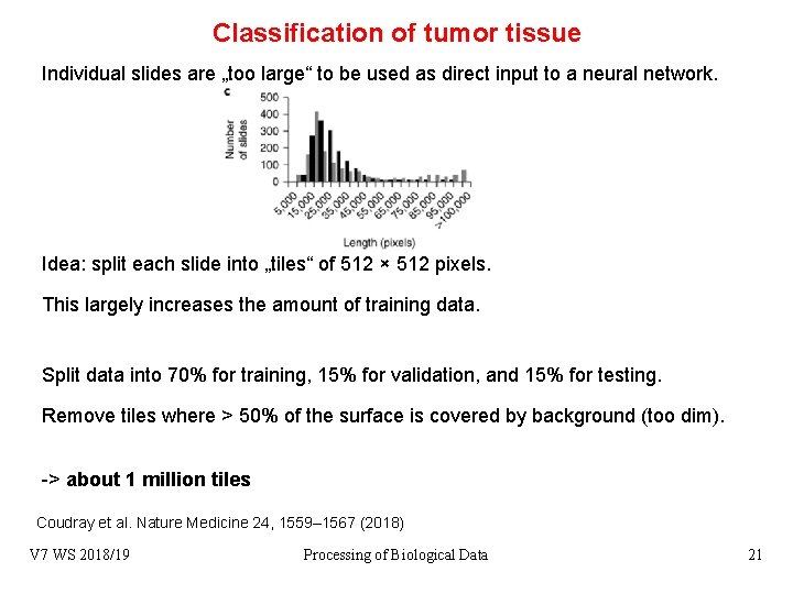
Classification of tumor tissue Individual slides are „too large“ to be used as direct input to a neural network. Idea: split each slide into „tiles“ of 512 × 512 pixels. This largely increases the amount of training data. Split data into 70% for training, 15% for validation, and 15% for testing. Remove tiles where > 50% of the surface is covered by background (too dim). -> about 1 million tiles Coudray et al. Nature Medicine 24, 1559– 1567 (2018) V 7 WS 2018/19 Processing of Biological Data 21

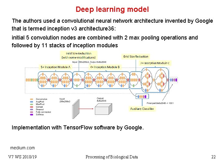
Deep learning model The authors used a convolutional neural network architecture invented by Google that is termed inception v 3 architecture 36: initial 5 convolution nodes are combined with 2 max pooling operations and followed by 11 stacks of inception modules Implementation with Tensor. Flow software by Google. medium. com V 7 WS 2018/19 Processing of Biological Data 22

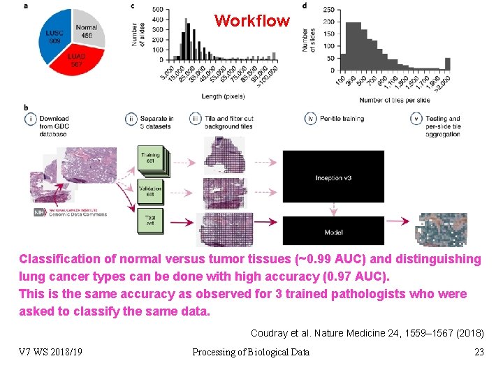
Workflow Classification of normal versus tumor tissues (~0. 99 AUC) and distinguishing lung cancer types can be done with high accuracy (0. 97 AUC). This is the same accuracy as observed for 3 trained pathologists who were asked to classify the same data. Coudray et al. Nature Medicine 24, 1559– 1567 (2018) V 7 WS 2018/19 Processing of Biological Data 23

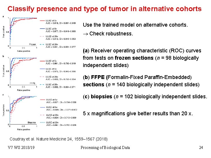
Classify presence and type of tumor in alternative cohorts Use the trained model on alternative cohorts. Check robustness. (a) Receiver operating characteristic (ROC) curves from tests on frozen sections (n = 98 biologically independent slides) (b) FFPE (Formalin-Fixed Paraffin-Embedded) sections (n = 140 biologically independent slides) (c) biopsies (n = 102 biologically independent slides. 5 x magnifications give better results than 20 x. Coudray et al. Nature Medicine 24, 1559– 1567 (2018) V 7 WS 2018/19 Processing of Biological Data 24

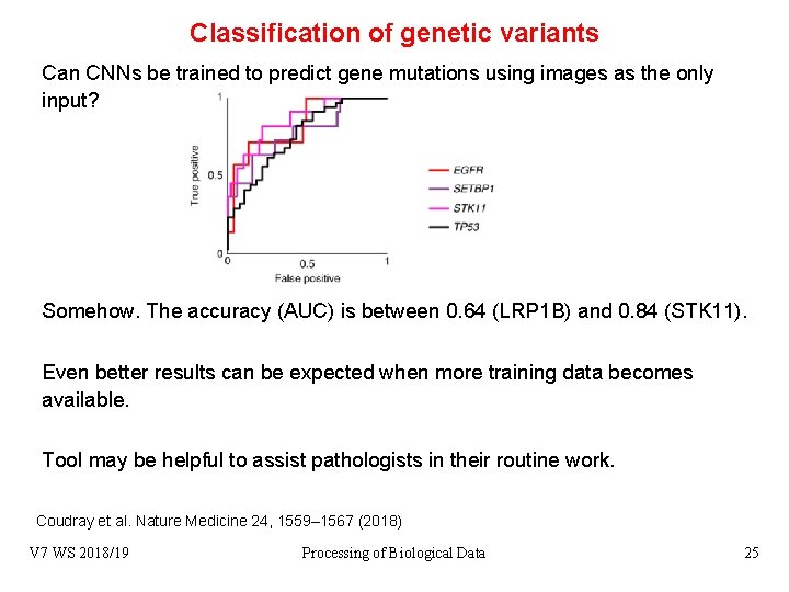
Classification of genetic variants Can CNNs be trained to predict gene mutations using images as the only input? Somehow. The accuracy (AUC) is between 0. 64 (LRP 1 B) and 0. 84 (STK 11). Even better results can be expected when more training data becomes available. Tool may be helpful to assist pathologists in their routine work. Coudray et al. Nature Medicine 24, 1559– 1567 (2018) V 7 WS 2018/19 Processing of Biological Data 25

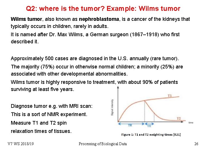
Q 2: where is the tumor? Example: Wilms tumor, also known as nephroblastoma, is a cancer of the kidneys that typically occurs in children, rarely in adults. It is named after Dr. Max Wilms, a German surgeon (1867– 1918) who first described it. Approximately 500 cases are diagnosed in the U. S. annually (rare tumor). The majority (75%) occur in otherwise normal children; a minority (25%) are associated with other developmental abnormalities. Wilms tumor is highly responsive to treatment, with about 90% of patients surviving at least five years. Diagnose tumor e. g. with MRI scan: This is a sort of NMR experiment. Measure T 1 and T 2 spin relaxation times of tissues. V 7 WS 2018/19 Processing of Biological Data 26

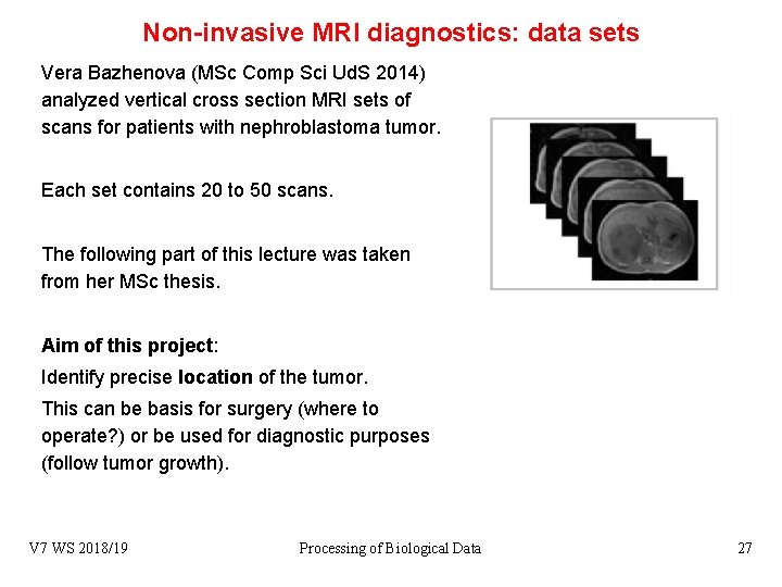
Non-invasive MRI diagnostics: data sets Vera Bazhenova (MSc Comp Sci Ud. S 2014) analyzed vertical cross section MRI sets of scans for patients with nephroblastoma tumor. Each set contains 20 to 50 scans. The following part of this lecture was taken from her MSc thesis. Aim of this project: Identify precise location of the tumor. This can be basis for surgery (where to operate? ) or be used for diagnostic purposes (follow tumor growth). V 7 WS 2018/19 Processing of Biological Data 27

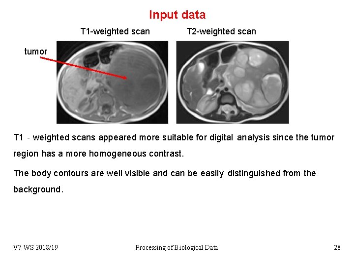
Input data T 1 -weighted scan T 2 -weighted scan tumor T 1‐weighted scans appeared more suitable for digital analysis since the tumor region has a more homogeneous contrast. The body contours are well visible and can be easily distinguished from the background. V 7 WS 2018/19 Processing of Biological Data 28

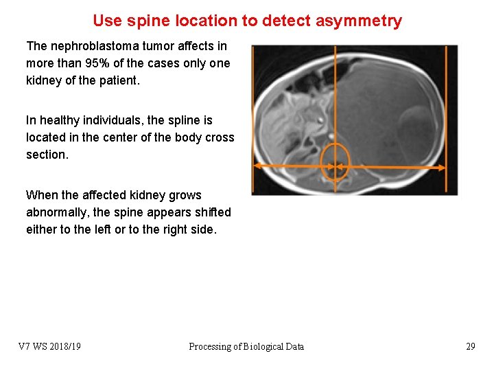
Use spine location to detect asymmetry The nephroblastoma tumor affects in more than 95% of the cases only one kidney of the patient. In healthy individuals, the spline is located in the center of the body cross section. When the affected kidney grows abnormally, the spine appears shifted either to the left or to the right side. V 7 WS 2018/19 Processing of Biological Data 29

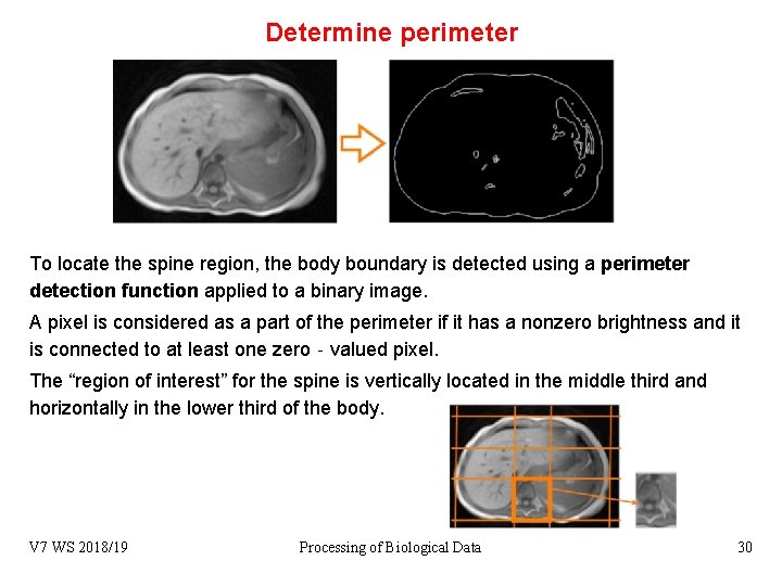
Determine perimeter To locate the spine region, the body boundary is detected using a perimeter detection function applied to a binary image. A pixel is considered as a part of the perimeter if it has a nonzero brightness and it is connected to at least one zero‐valued pixel. The “region of interest” for the spine is vertically located in the middle third and horizontally in the lower third of the body. V 7 WS 2018/19 Processing of Biological Data 30

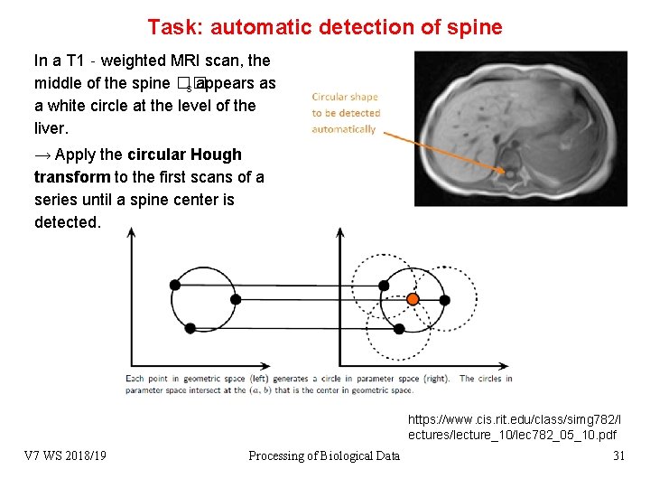
Task: automatic detection of spine In a T 1‐weighted MRI scan, the middle of the spine �� s appears as a white circle at the level of the liver. → Apply the circular Hough transform to the first scans of a series until a spine center is detected. https: //www. cis. rit. edu/class/simg 782/l ectures/lecture_10/lec 782_05_10. pdf V 7 WS 2018/19 Processing of Biological Data 31

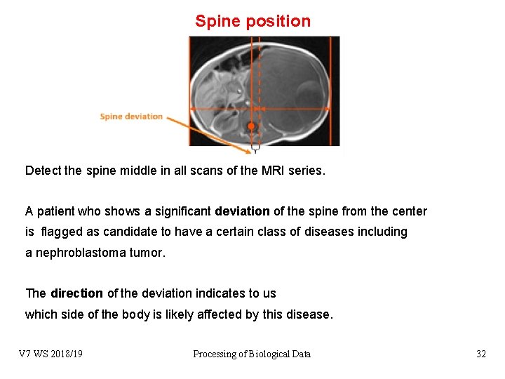
Spine position Detect the spine middle in all scans of the MRI series. A patient who shows a significant deviation of the spine from the center is flagged as candidate to have a certain class of diseases including a nephroblastoma tumor. The direction of the deviation indicates to us which side of the body is likely affected by this disease. V 7 WS 2018/19 Processing of Biological Data 32

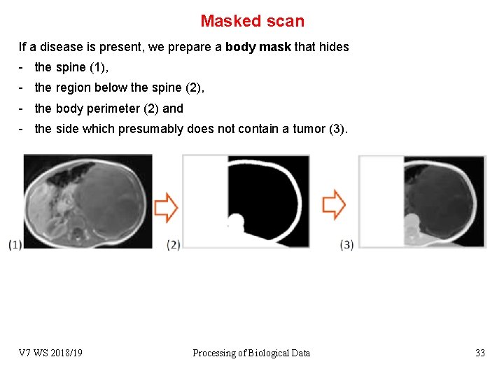
Masked scan If a disease is present, we prepare a body mask that hides - the spine (1), - the region below the spine (2), - the body perimeter (2) and - the side which presumably does not contain a tumor (3). V 7 WS 2018/19 Processing of Biological Data 33

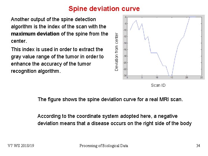
Another output of the spine detection algorithm is the index of the scan with the maximum deviation of the spine from the center. This index is used in order to extract the gray value range of the tumor in order to enhance the accuracy of the tumor recognition algorithm. Deviation from center Spine deviation curve Scan ID The figure shows the spine deviation curve for a real MRI scan. According to the coordinate system adopted here, a negative deviation means that a disease occurs on the right side of the body V 7 WS 2018/19 Processing of Biological Data 34

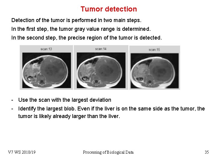
Tumor detection Detection of the tumor is performed in two main steps. In the first step, the tumor gray value range is determined. In the second step, the precise region of the tumor is detected. - Use the scan with the largest deviation - Identify the largest blob. Even if the liver is on the same side as the tumor, the tumor is likely already larger than the liver. V 7 WS 2018/19 Processing of Biological Data 35

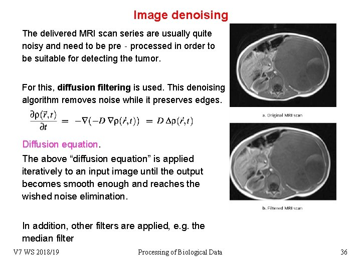
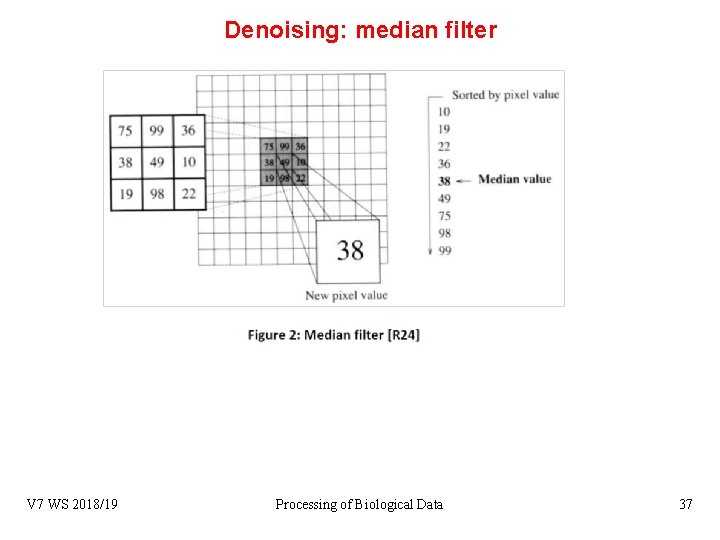
Image denoising The delivered MRI scan series are usually quite noisy and need to be pre‐processed in order to be suitable for detecting the tumor. For this, diffusion filtering is used. This denoising algorithm removes noise while it preserves edges. Diffusion equation. The above “diffusion equation” is applied iteratively to an input image until the output becomes smooth enough and reaches the wished noise elimination. In addition, other filters are applied, e. g. the median filter V 7 WS 2018/19 Processing of Biological Data 36

Denoising: median filter V 7 WS 2018/19 Processing of Biological Data 37

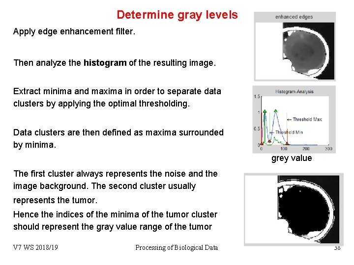
Determine gray levels Apply edge enhancement filter. Then analyze the histogram of the resulting image. Extract minima and maxima in order to separate data clusters by applying the optimal thresholding. Data clusters are then defined as maxima surrounded by minima. grey value The first cluster always represents the noise and the image background. The second cluster usually represents the tumor. Hence the indices of the minima of the tumor cluster should represent the gray value range of the tumor V 7 WS 2018/19 Processing of Biological Data 38

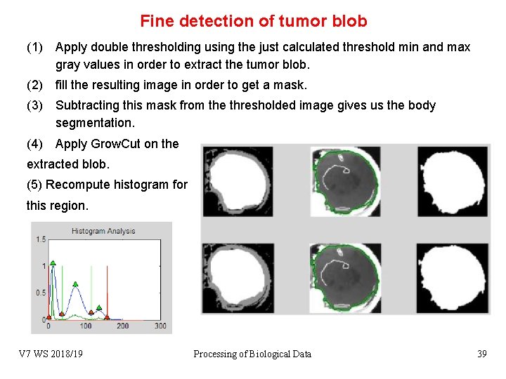
Fine detection of tumor blob (1) Apply double thresholding using the just calculated threshold min and max gray values in order to extract the tumor blob. (2) fill the resulting image in order to get a mask. (3) Subtracting this mask from the thresholded image gives us the body segmentation. (4) Apply Grow. Cut on the extracted blob. (5) Recompute histogram for this region. V 7 WS 2018/19 Processing of Biological Data 39

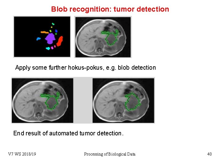
Blob recognition: tumor detection Apply some further hokus-pokus, e. g. blob detection End result of automated tumor detection. V 7 WS 2018/19 Processing of Biological Data 40

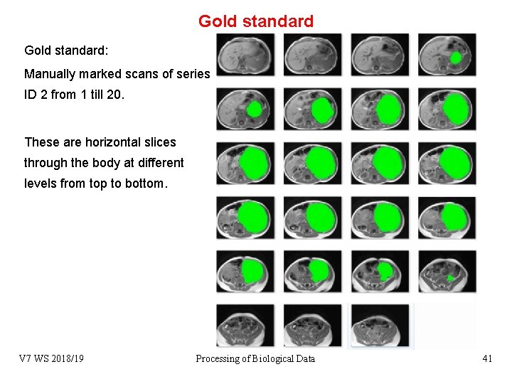
Gold standard: Manually marked scans of series ID 2 from 1 till 20. These are horizontal slices through the body at different levels from top to bottom. V 7 WS 2018/19 Processing of Biological Data 41

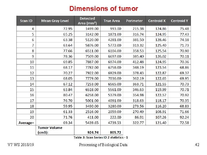
Dimensions of tumor Blob recognition V 7 WS 2018/19 Processing of Biological Data 42