Introduction to MRI Physics Ian Miller July 11

Introduction to MRI Physics Ian Miller July 11, 2007

Goal of Today’s Lecture • Relate the concepts of MRI physics to things that engineers and neurophysiologists already understand • Lay the groundwork for more detailed understanding of more complicated imaging techniques • • • Fast spin echo Echo planar imaging Volume imaging 3 D time of flight Diffusion …

Why this is an Intimidating Topic • There a myriad of basic physics principles involved, each of which is individually important and hard to skip over • Need to simultaneously consider two scales • single particles • aggregates of billions of particles • There are multiple dimensions involved to keep straight • The math is complicated for non-engineers, and most of it is vector-based • It’s easy to convince yourself you “get it”

Organization of Discussion • • Review of Relevant Basic Physical Principles Magnetism Resonance Image Creation T 1 and T 2 Anatomy of an MR Scanner Future Topics

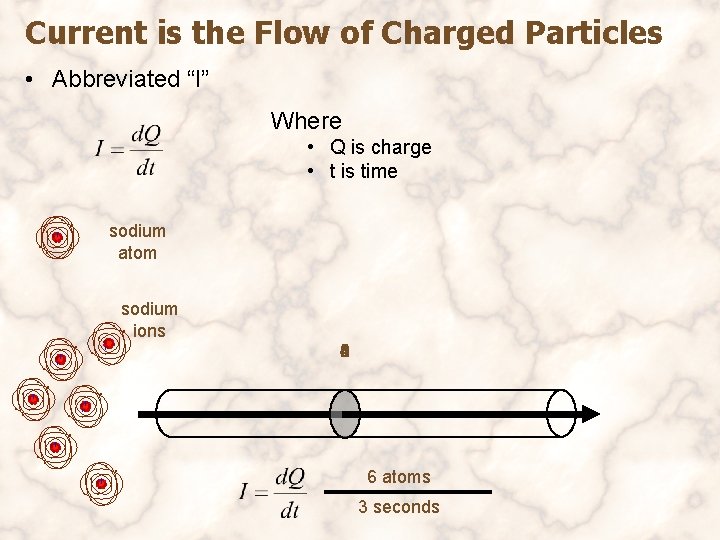
Current is the Flow of Charged Particles • Abbreviated “I” Where • Q is charge • t is time sodium atom sodium ions 6 5 4 3 2 1 6 atoms 3 seconds

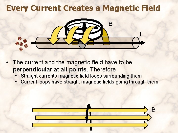
Every Current Creates a Magnetic Field B I • The current and the magnetic field have to be perpendicular at all points. Therefore • Straight currents magnetic field loops surrounding them • Current loops have straight magnetic fields going through them I B

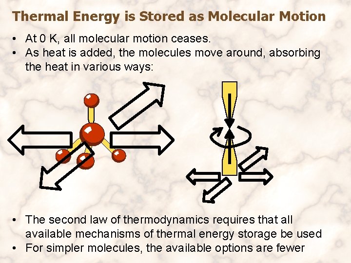
Thermal Energy is Stored as Molecular Motion • At 0 K, all molecular motion ceases. • As heat is added, the molecules move around, absorbing the heat in various ways: • The second law of thermodynamics requires that all available mechanisms of thermal energy storage be used • For simpler molecules, the available options are fewer

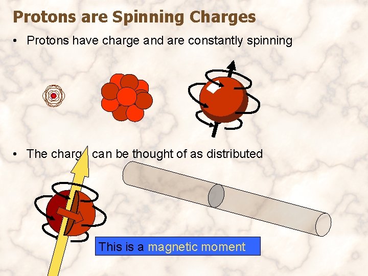
Protons are Spinning Charges • Protons have charge and are constantly spinning • The charge can be thought of as distributed This is a magnetic moment

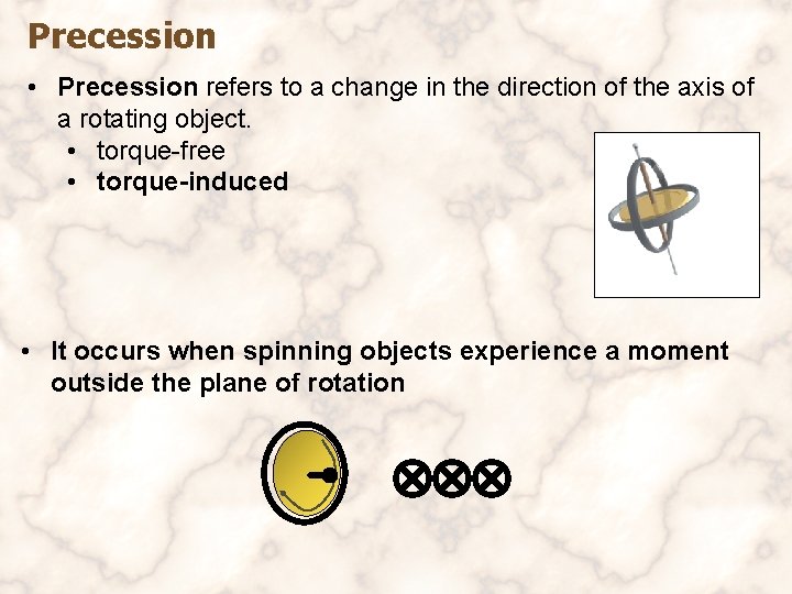
Precession • Precession refers to a change in the direction of the axis of a rotating object. • torque-free • torque-induced • It occurs when spinning objects experience a moment outside the plane of rotation

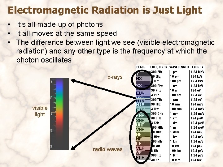
Electromagnetic Radiation is Just Light • It’s all made up of photons • It all moves at the same speed • The difference between light we see (visible electromagnetic radiation) and any other type is the frequency at which the photon oscillates x-rays visible light radio waves

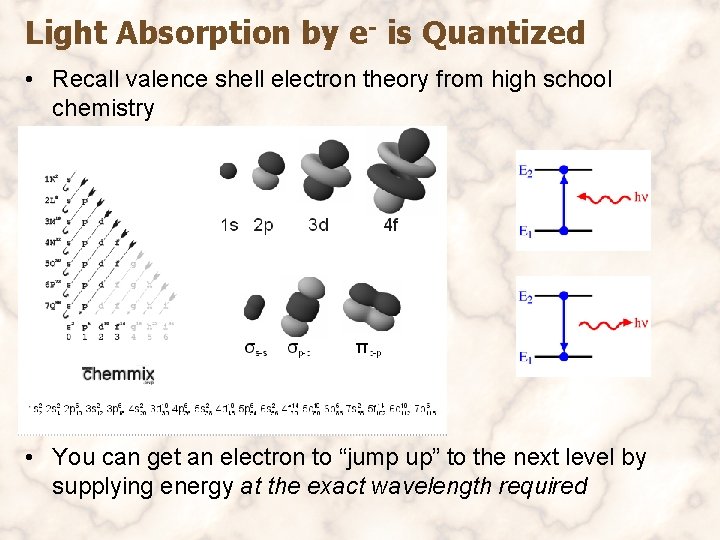
Light Absorption by e- is Quantized • Recall valence shell electron theory from high school chemistry • You can get an electron to “jump up” to the next level by supplying energy at the exact wavelength required

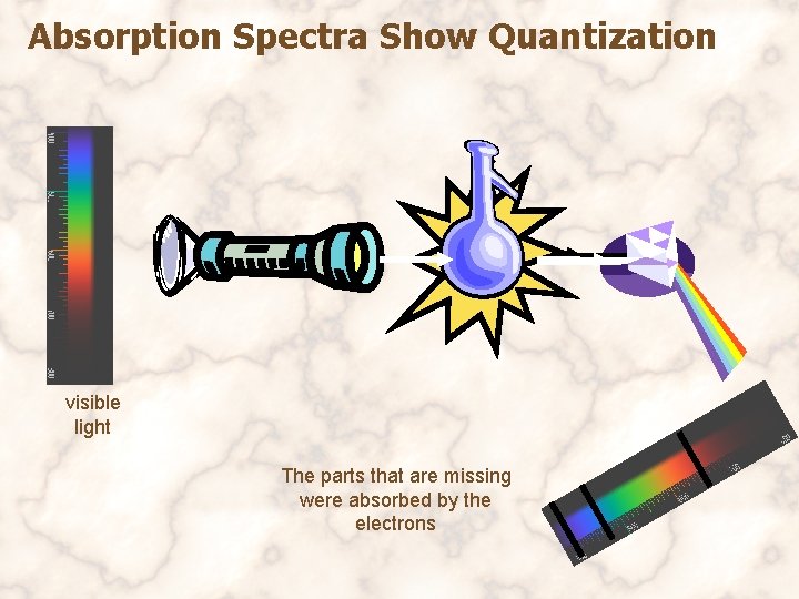
Absorption Spectra Show Quantization visible light The parts that are missing were absorbed by the electrons

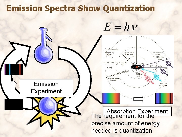
Emission Spectra Show Quantization Emission Experiment Absorption Experiment The requirement for the precise amount of energy needed is quantization

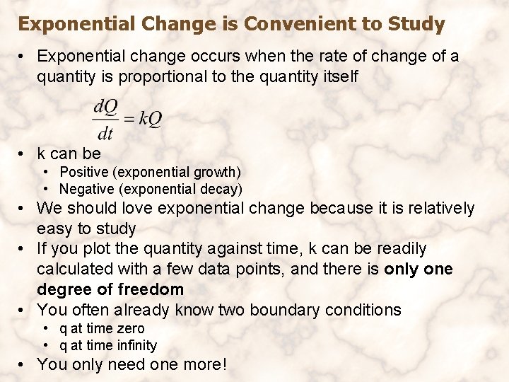
Exponential Change is Convenient to Study • Exponential change occurs when the rate of change of a quantity is proportional to the quantity itself • k can be • Positive (exponential growth) • Negative (exponential decay) • We should love exponential change because it is relatively easy to study • If you plot the quantity against time, k can be readily calculated with a few data points, and there is only one degree of freedom • You often already know two boundary conditions • q at time zero • q at time infinity • You only need one more!

Recap of Review Material • Current is the Flow of Charged Particles • Every Current Creates a Magnetic Field • Perpendicular at all points to the current • Thermal Energy is Stored as Molecular Motion • Protons are Spinning Charges • Protons have a current loop • Protons have a magnetic moment along the axis of rotation • Precession • Occurs when a spinning object experiences a moment out of the plane of rotation • • • Electromagnetic Radiation is Just Light Absorption by particles is Quantized Absorption Spectra Show Quantization Emission Spectra Show Quantization Exponential Change is Convenient to Study Now we need to scale up to the bulk / macroscopic scale

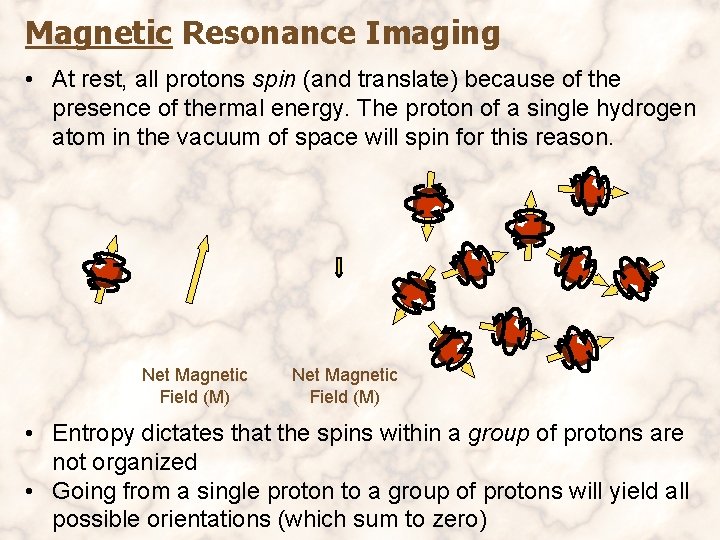
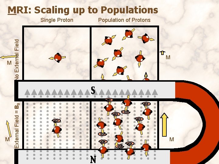
Magnetic Resonance Imaging • At rest, all protons spin (and translate) because of the presence of thermal energy. The proton of a single hydrogen atom in the vacuum of space will spin for this reason. Net Magnetic Field (M) • Entropy dictates that the spins within a group of protons are not organized • Going from a single proton to a group of protons will yield all possible orientations (which sum to zero)

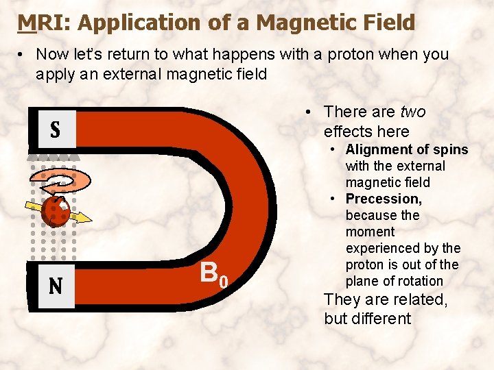
MRI: Application of a Magnetic Field • Now let’s return to what happens with a proton when you apply an external magnetic field • There are two effects here B 0 • Alignment of spins with the external magnetic field • Precession, because the moment experienced by the proton is out of the plane of rotation They are related, but different

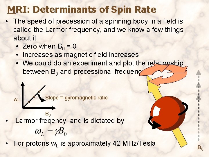
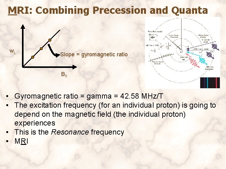
MRI: Determinants of Spin Rate • The speed of precession of a spinning body in a field is called the Larmor frequency, and we know a few things about it • Zero when B 0 = 0 • Increases as magnetic field increases • We could do an experiment and plot the relationship between B 0 and precessional frequency w. L • Slope = gyromagnetic ratio B 0 Larmor freqency, and is dictated by • For protons w. L is approximately 42 MHz/Tesla B 0

MRI: Scaling up to Populations M External Field = B 0 M No External Field Single Proton Population of Protons M M

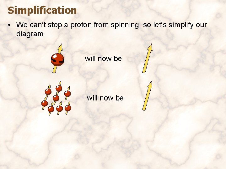
Simplification • We can’t stop a proton from spinning, so let’s simplify our diagram will now be

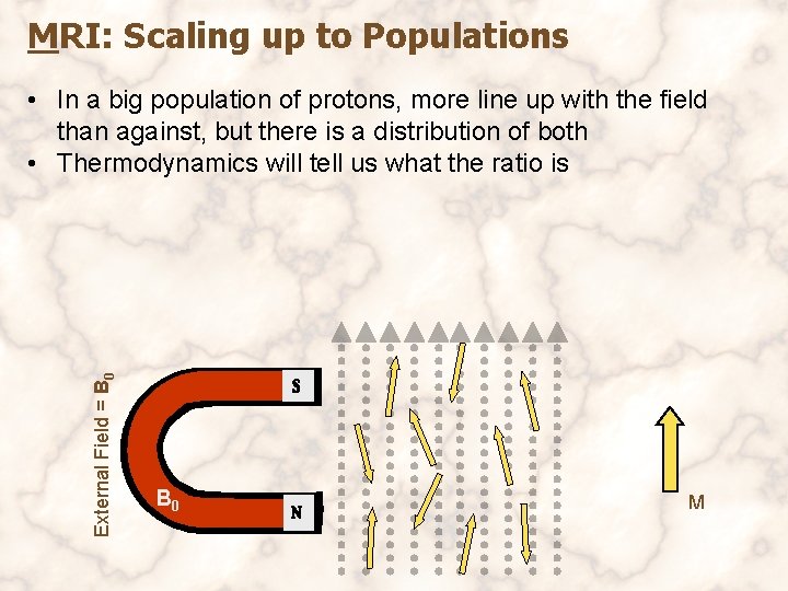
MRI: Scaling up to Populations External Field = B 0 • In a big population of protons, more line up with the field than against, but there is a distribution of both • Thermodynamics will tell us what the ratio is B 0 M

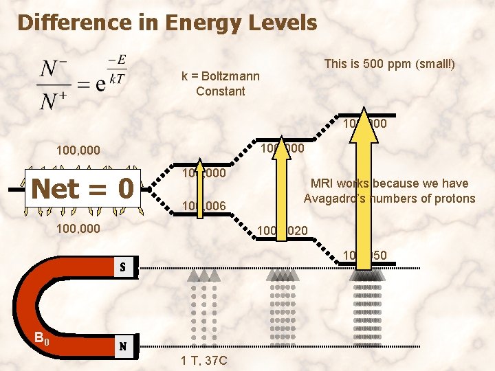
Difference in Energy Levels This is 500 ppm (small!) k = Boltzmann Constant 100, 000 Net = 0 100, 006 100, 000 MRI works because we have Avagadro’s numbers of protons 100, 0020 100, 050 B 0 1 T, 37 C

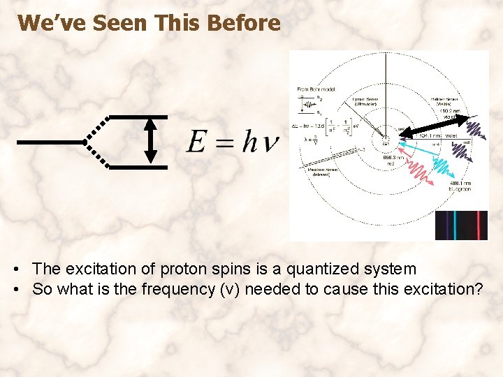
We’ve Seen This Before • The excitation of proton spins is a quantized system • So what is the frequency (v) needed to cause this excitation?

MRI: Combining Precession and Quanta w. L Slope = gyromagnetic ratio B 0 • Gyromagnetic ratio = gamma = 42. 58 MHz/T • The excitation frequency (for an individual proton) is going to depend on the magnetic field (the individual proton) experiences • This is the Resonance frequency • MRI

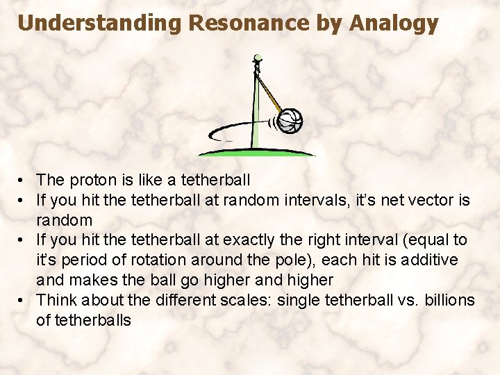
Understanding Resonance by Analogy • The proton is like a tetherball • If you hit the tetherball at random intervals, it’s net vector is random • If you hit the tetherball at exactly the right interval (equal to it’s period of rotation around the pole), each hit is additive and makes the ball go higher and higher • Think about the different scales: single tetherball vs. billions of tetherballs

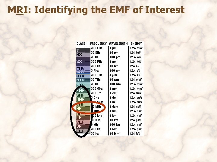
MRI: Identifying the EMF of Interest

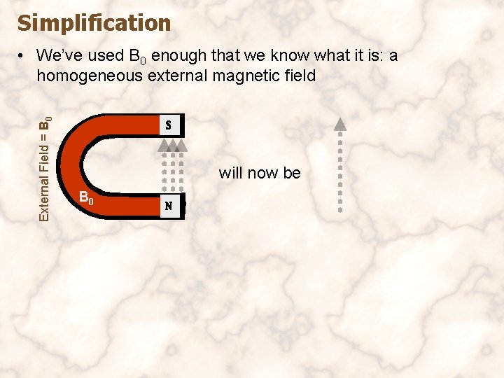
Simplification External Field = B 0 • We’ve used B 0 enough that we know what it is: a homogeneous external magnetic field will now be B 0

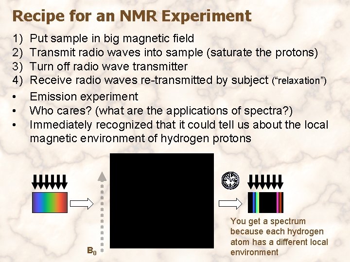
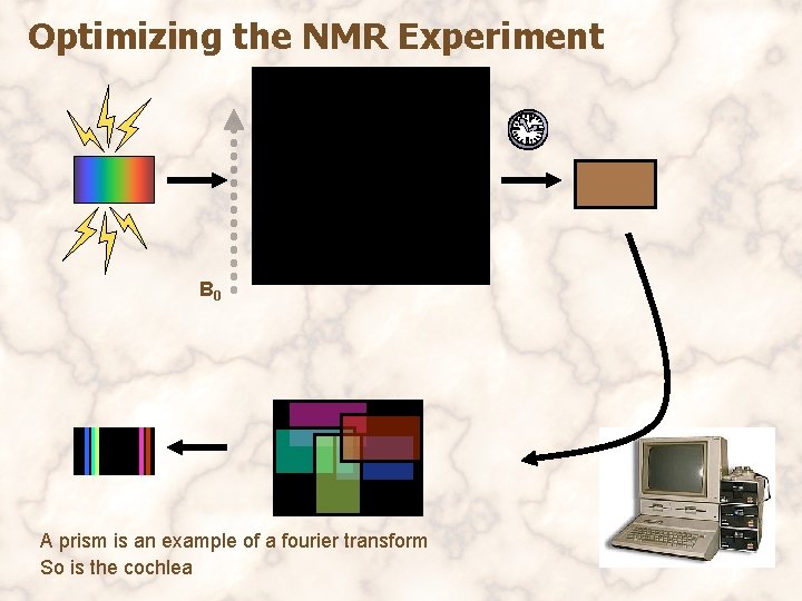
Recipe for an NMR Experiment 1) 2) 3) 4) • • • Put sample in big magnetic field Transmit radio waves into sample (saturate the protons) Turn off radio wave transmitter Receive radio waves re-transmitted by subject (“relaxation”) Emission experiment Who cares? (what are the applications of spectra? ) Immediately recognized that it could tell us about the local magnetic environment of hydrogen protons B 0 You get a spectrum because each hydrogen atom has a different local environment

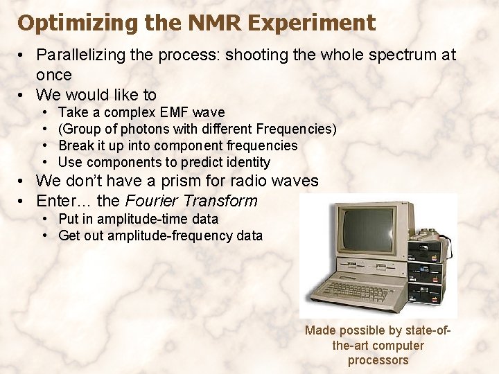
Optimizing the NMR Experiment • Parallelizing the process: shooting the whole spectrum at once • We would like to • • Take a complex EMF wave (Group of photons with different Frequencies) Break it up into component frequencies Use components to predict identity • We don’t have a prism for radio waves • Enter… the Fourier Transform • Put in amplitude-time data • Get out amplitude-frequency data Made possible by state-ofthe-art computer processors

Optimizing the NMR Experiment B 0 A prism is an example of a fourier transform So is the cochlea

Lauterbur’s Insight • Conventional NMR used spectra to make inferences about local magnetic perturbations in a uniform magnetic field • If the magnetic field was instead made to vary with position, then the resonant frequency spectrum would instead tell you about location in a uniform population of protons • Great idea…

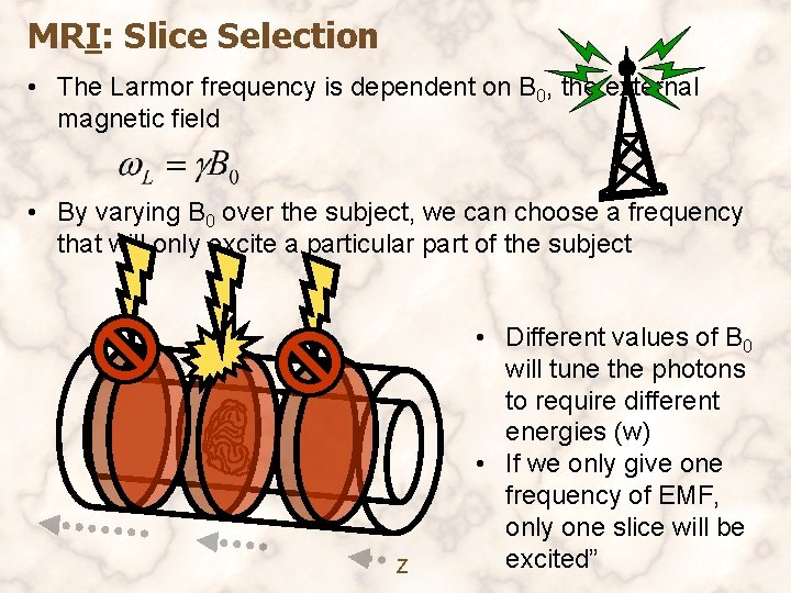
MRI: Slice Selection • The Larmor frequency is dependent on B 0, the external magnetic field • By varying B 0 over the subject, we can choose a frequency that will only excite a particular part of the subject Z • Different values of B 0 will tune the photons to require different energies (w) • If we only give one frequency of EMF, only one slice will be excited”

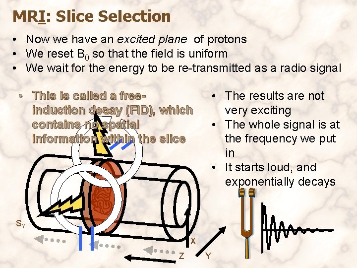
MRI: Slice Selection • Now we have an excited plane of protons • We reset B 0 so that the field is uniform • We wait for the energy to be re-transmitted as a radio signal • This is called a free. SX induction decay (FID), which contains no spatial information within the slice • The results are not very exciting • The whole signal is at the frequency we put in • It starts loud, and exponentially decays SY X Z Y

Questions?

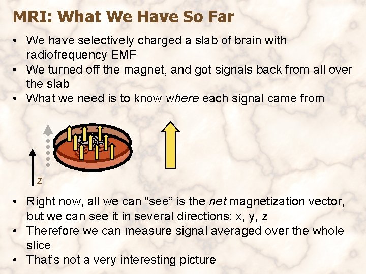
MRI: What We Have So Far • We have selectively charged a slab of brain with radiofrequency EMF • We turned off the magnet, and got signals back from all over the slab • What we need is to know where each signal came from Z • Right now, all we can “see” is the net magnetization vector, but we can see it in several directions: x, y, z • Therefore we can measure signal averaged over the whole slice • That’s not a very interesting picture

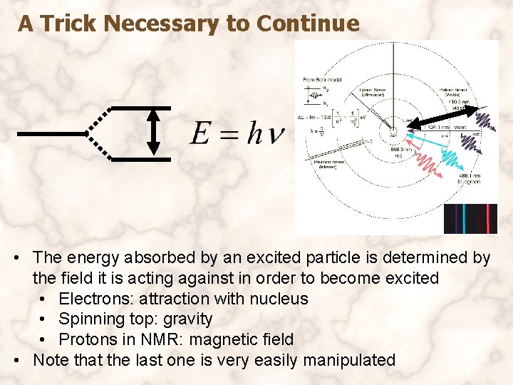
A Trick Necessary to Continue • The energy absorbed by an excited particle is determined by the field it is acting against in order to become excited • Electrons: attraction with nucleus • Spinning top: gravity • Protons in NMR: magnetic field • Note that the last one is very easily manipulated

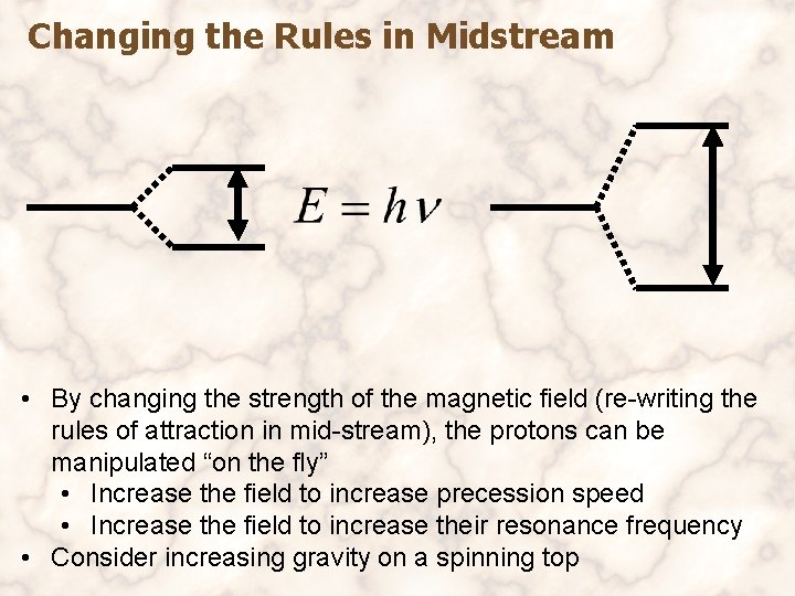
Changing the Rules in Midstream • By changing the strength of the magnetic field (re-writing the rules of attraction in mid-stream), the protons can be manipulated “on the fly” • Increase the field to increase precession speed • Increase the field to increase their resonance frequency • Consider increasing gravity on a spinning top

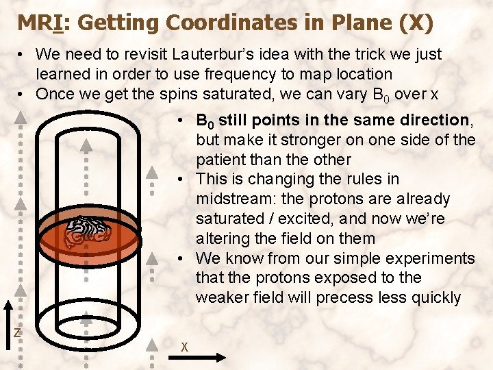
MRI: Getting Coordinates in Plane (X) • We need to revisit Lauterbur’s idea with the trick we just learned in order to use frequency to map location • Once we get the spins saturated, we can vary B 0 over x • B 0 still points in the same direction, but make it stronger on one side of the patient than the other • This is changing the rules in midstream: the protons are already saturated / excited, and now we’re altering the field on them • We know from our simple experiments that the protons exposed to the weaker field will precess less quickly Z X

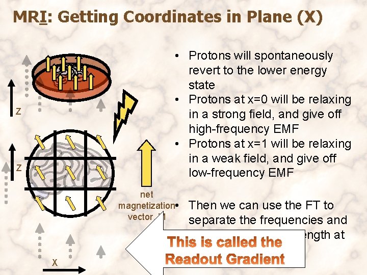
MRI: Getting Coordinates in Plane (X) • Protons will spontaneously revert to the lower energy state • Protons at x=0 will be relaxing in a strong field, and give off high-frequency EMF • Protons at x=1 will be relaxing in a weak field, and give off low-frequency EMF Z Z net magnetization • vector, M X Then we can use the FT to separate the frequencies and identify the signal strength at each x-coordinate

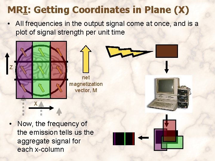
MRI: Getting Coordinates in Plane (X) • All frequencies in the output signal come at once, and is a plot of signal strength per unit time Z net magnetization vector, M X • Now, the frequency of the emission tells us the aggregate signal for each x-column

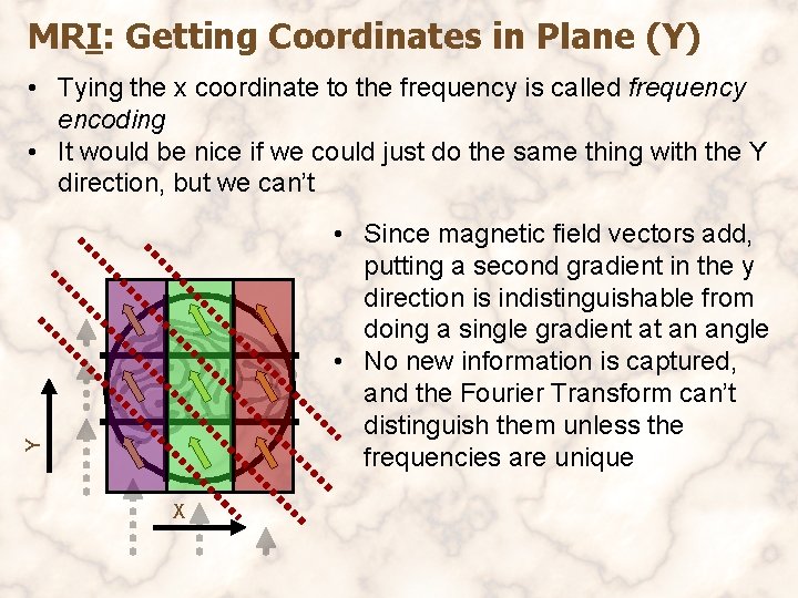
MRI: Getting Coordinates in Plane (Y) • Tying the x coordinate to the frequency is called frequency encoding • It would be nice if we could just do the same thing with the Y direction, but we can’t Y • Since magnetic field vectors add, putting a second gradient in the y direction is indistinguishable from doing a single gradient at an angle • No new information is captured, and the Fourier Transform can’t distinguish them unless the frequencies are unique X

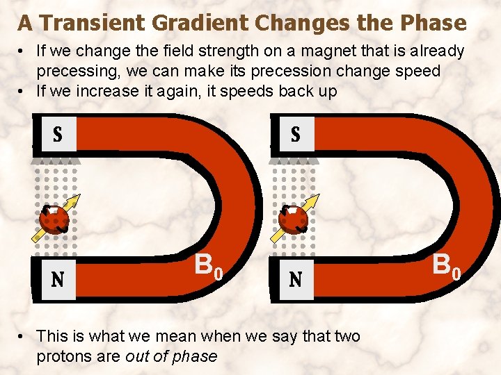
A Transient Gradient Changes the Phase • If we change the field strength on a magnet that is already precessing, we can make its precession change speed • If we increase it again, it speeds back up B 0 • This is what we mean when we say that two protons are out of phase B 0

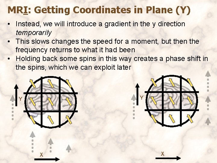
MRI: Getting Coordinates in Plane (Y) • Instead, we will introduce a gradient in the y direction temporarily • This slows changes the speed for a moment, but then the frequency returns to what it had been • Holding back some spins in this way creates a phase shift in the spins, which we can exploit later Y Y X X

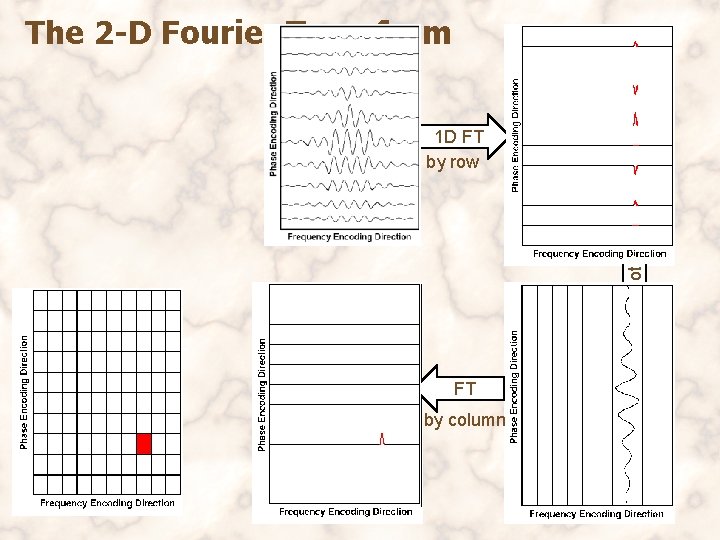
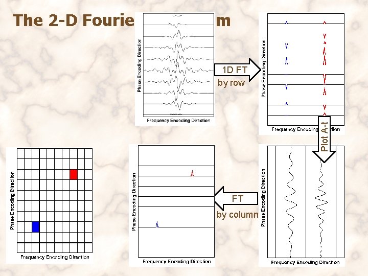
MRI: Getting Coordinates in Plane (Y) • This technique gives us an extra degree of freedom • The Fourier transform does not know how to process phase information, but it does preserve it • We then do a second Fourier transform in order to obtain the information we want • Let’s use an example to understand the 2 D Fourier Transform

The 2 -D Fourier Transform Plot A-t 1 D FT by row FT by column

The 2 -D Fourier Transform Plot A-t 1 D FT by row FT by column

MRI: What we End Up With • We now have a plot of signal as a function of time at each individual voxel • We know that the signal will decay unequally in different tissues, so we get signal-vs-position plots at multiple time points, calculate the rate of decay, and give that pixel a shade near white if the decay constant is large, and a shade near black if the decay constant is short • In actuality, the phase-encoding step is done first, because the magnetic gradient it requires is transient. The frequencyencoding step is done last, because it needs to be active when the protons relax (…the readout gradient)

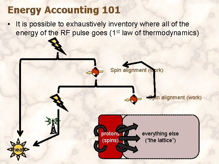
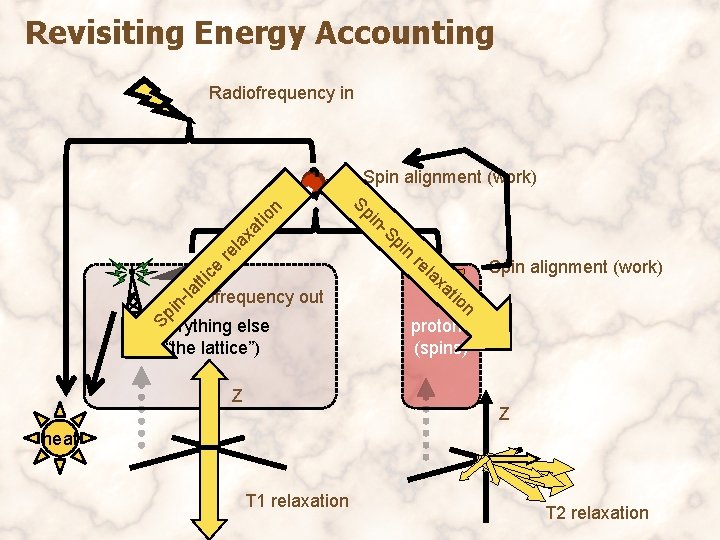
Energy Accounting 101 • It is possible to exhaustively inventory where all of the energy of the RF pulse goes (1 st law of thermodynamics) Spin alignment (work) protons the everything universe else the physicist) lattice”) (spins)(as seen by(“the heat

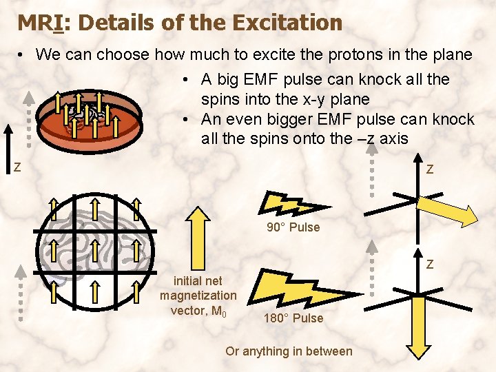
MRI: Details of the Excitation • We can choose how much to excite the protons in the plane • A big EMF pulse can knock all the spins into the x-y plane • An even bigger EMF pulse can knock all the spins onto the –z axis Z Z 90° Pulse Z initial net magnetization vector, M 0 180° Pulse Or anything in between

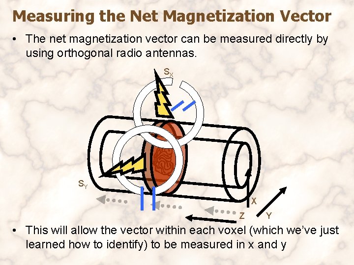
Measuring the Net Magnetization Vector • The net magnetization vector can be measured directly by using orthogonal radio antennas. SX SY X Z Y • This will allow the vector within each voxel (which we’ve just learned how to identify) to be measured in x and y

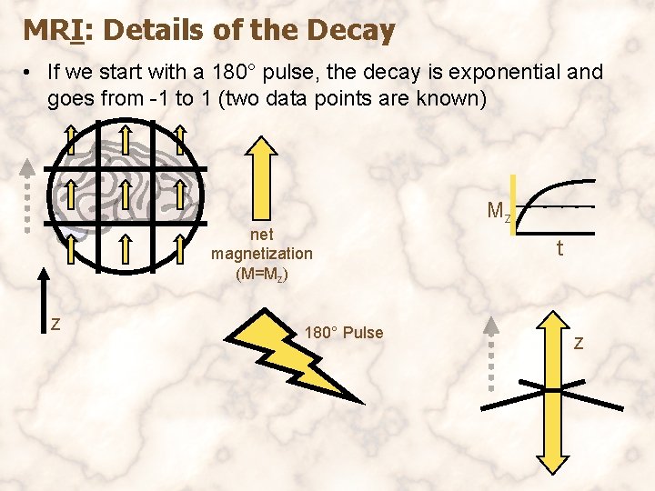
MRI: Details of the Decay • If we start with a 180° pulse, the decay is exponential and goes from -1 to 1 (two data points are known) net magnetization (M=Mz) Z 180° Pulse Mz t Z

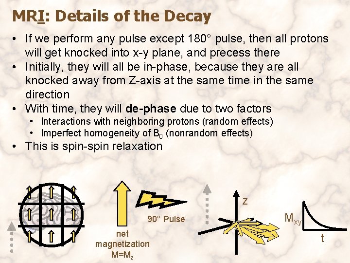
MRI: Details of the Decay • If we perform any pulse except 180° pulse, then all protons will get knocked into x-y plane, and precess there • Initially, they will all be in-phase, because they are all knocked away from Z-axis at the same time in the same direction • With time, they will de-phase due to two factors • Interactions with neighboring protons (random effects) • Imperfect homogeneity of B 0 (nonrandom effects) • This is spin-spin relaxation Z 90° Pulse net magnetization M=Mz Mxy t

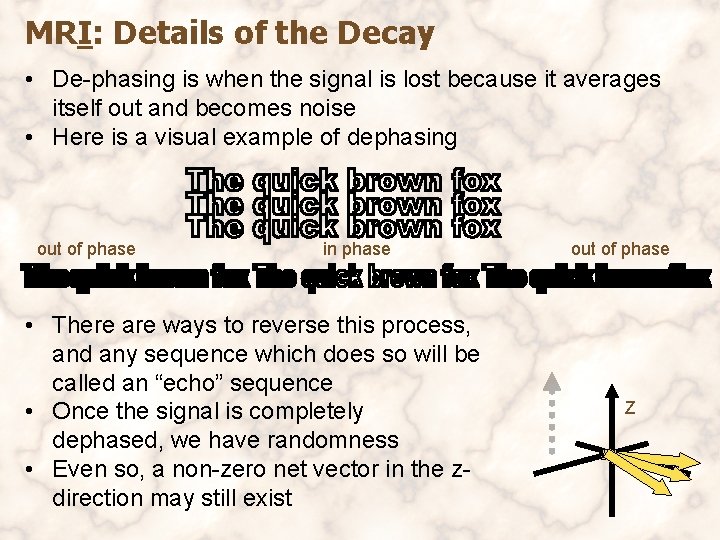
MRI: Details of the Decay • De-phasing is when the signal is lost because it averages itself out and becomes noise • Here is a visual example of dephasing out of phase in phase • There are ways to reverse this process, and any sequence which does so will be called an “echo” sequence • Once the signal is completely dephased, we have randomness • Even so, a non-zero net vector in the zdirection may still exist out of phase Z

Revisiting Energy Accounting Radiofrequency in Spin alignment (work) ti a x ce on la re ti t Radiofrequency out -la n i Sp everything else (“the lattice”) Z Sp in -S pi n re la xa Spin alignment (work) t io n protons (spins) Z heat T 1 relaxation T 2 relaxation

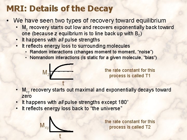
MRI: Details of the Decay • We have seen two types of recovery toward equilibrium • Mz recovery starts out low and recovers exponentially back toward one (because z equilbrium is to line back up with B 0) • It happens with all pulse strengths • It reflects energy loss to surrounding molecules • Random interactions (changes moment to moment, “noise”) • Nonrandom interactions (is static for a given molecule, “bias”) the rate constant for this process is called T 1 Mz t • Mxy recovery starts out maximal and exponentially decays toward zero • It happens with all pulse strengths except 180° • It reflects energy loss back to “the universe” the rate constant for this process is called T 2 Mxy t

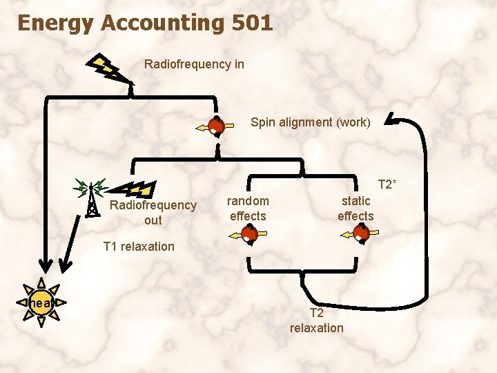
Energy Accounting 501 Radiofrequency in Spin alignment (work) T 2* Radiofrequency out random effects static effects T 1 relaxation heat T 2 relaxation

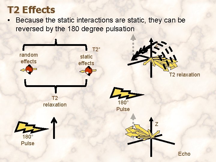
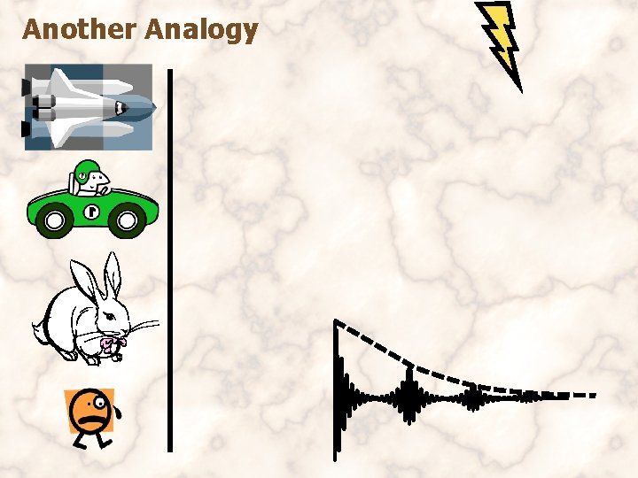
T 2 Effects • Because the static interactions are static, they can be reversed by the 180 degree pulsation Z T 2* static effects random effects T 2 relaxation 180° Pulse Z 180° Pulse Echo

Another Analogy

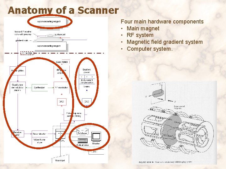
Anatomy of a Scanner Four main hardware components • Main magnet • RF system • Magnetic field gradient system • Computer system.

What We’ve Covered • Reviewed the most fundamental rules that govern MR phenomena • Identified how to excite selected photons using supermagnets and radio waves • Identified how to manipulate the excited photons in order to “encode” positional information • Frequency encoding • Phase encoding • Become familiar with 2 D Fourier transforms

Future Topics to Explore • Mechanisms of contrast • Proton Density • T 1, T 2* in more detail • Anisotropy • Flow • Diffusion • Tensor mapping • IV Contrast • Pulse Sequence Diagram Interpretation • Sequence selection, costs and benefits