Time Series Cross Sectional Pooled Data 1 Time

Time Series, Cross Sectional & Pooled Data • 1. Time Series Data -One location’s data across time -Yearly, monthly, quarterly (every three months), weekly, daily, etc. -ie: Canadian GDP, Enron stock value, your height, U of A tuition, world pop.

Time Series, Cross Sectional & Pooled Data • 2. Cross-Sectional Data -Multiple Locations at one time -Taken at same time (September report, January report, etc. ) -ie: stock portfolio, player stats, provincial GDP comparison, grade report

Time Series, Cross Sectional & Pooled Data • 3. Pooled Data -Combination of Time Series and Crosssectional Data -More difficult to use -Often required due to data restrictions

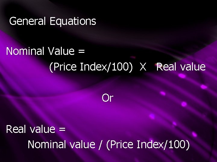
General Equations Nominal Value = (Price Index/100) X Real value Or Real value = Nominal value / (Price Index/100)

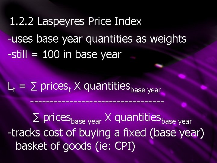
1. 2. 2 Laspeyres Price Index -uses base year quantities as weights -still = 100 in base year Lt = ∑ pricest X quantitiesbase year -----------------∑ pricesbase year X quantitiesbase year -tracks cost of buying a fixed (base year) basket of goods (ie: CPI)

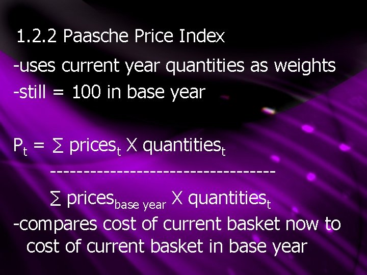
1. 2. 2 Paasche Price Index -uses current year quantities as weights -still = 100 in base year Pt = ∑ pricest X quantitiest -----------------∑ pricesbase year X quantitiest -compares cost of current basket now to cost of current basket in base year

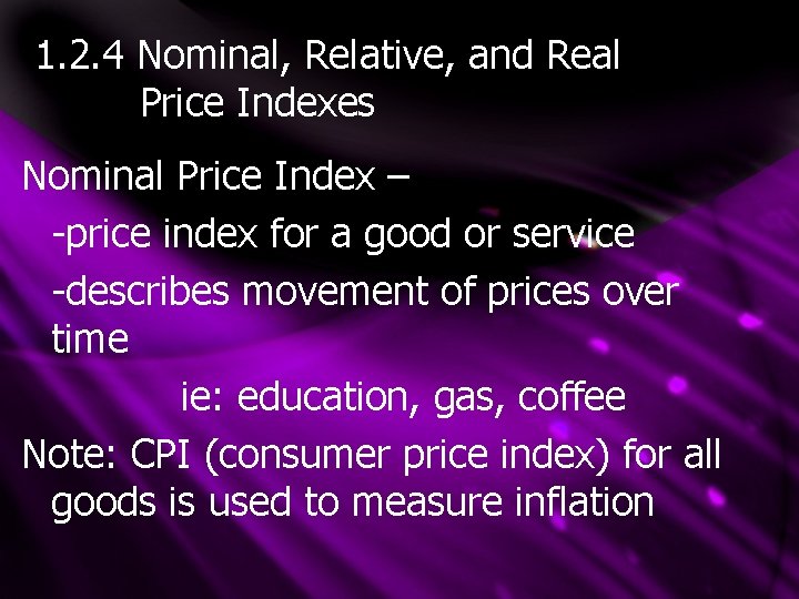
1. 2. 4 Nominal, Relative, and Real Price Indexes Nominal Price Index – -price index for a good or service -describes movement of prices over time ie: education, gas, coffee Note: CPI (consumer price index) for all goods is used to measure inflation

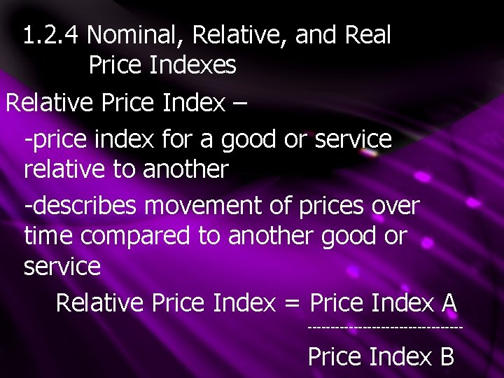
1. 2. 4 Nominal, Relative, and Real Price Indexes Relative Price Index – -price index for a good or service relative to another -describes movement of prices over time compared to another good or service Relative Price Index = Price Index A ----------------- Price Index B

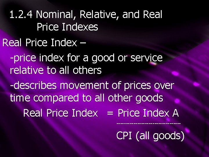
1. 2. 4 Nominal, Relative, and Real Price Indexes Real Price Index – -price index for a good or service relative to all others -describes movement of prices over time compared to all other goods Real Price Index = Price Index A ----------------- CPI (all goods)

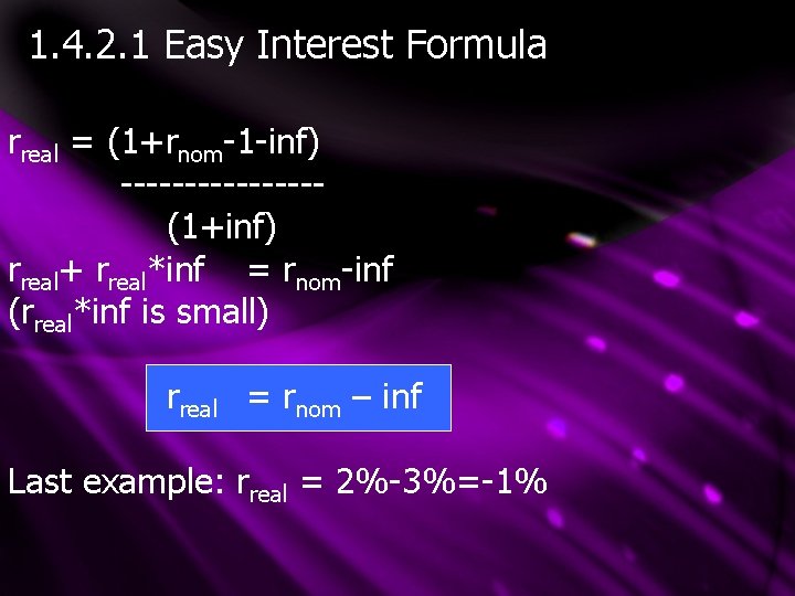
1. 4. 2. 1 Easy Interest Formula rreal = (1+rnom-1 -inf) --------(1+inf) rreal+ rreal*inf = rnom-inf (rreal*inf is small) rreal = rnom – inf Last example: rreal = 2%-3%=-1%

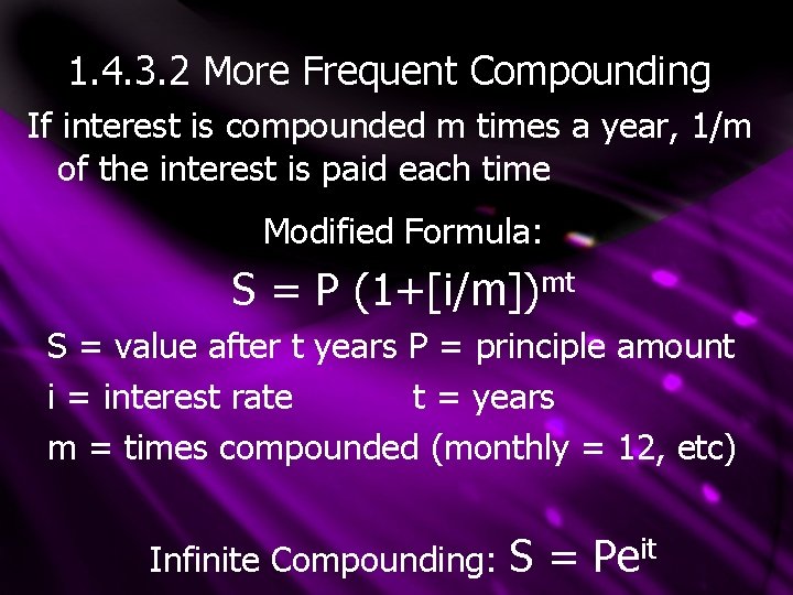
1. 4. 3. 2 More Frequent Compounding If interest is compounded m times a year, 1/m of the interest is paid each time Modified Formula: S = P (1+[i/m])mt S = value after t years P = principle amount i = interest rate t = years m = times compounded (monthly = 12, etc) Infinite Compounding: S = Peit

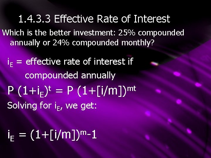
1. 4. 3. 3 Effective Rate of Interest Which is the better investment: 25% compounded annually or 24% compounded monthly? i. E = effective rate of interest if compounded annually P (1+i. E)t = P (1+[i/m])mt Solving for i. E, we get: i. E = (1+[i/m])m-1

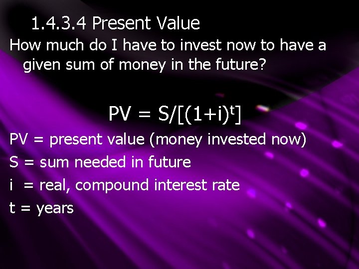
1. 4. 3. 4 Present Value How much do I have to invest now to have a given sum of money in the future? PV = S/[(1+i)t] PV = present value (money invested now) S = sum needed in future i = real, compound interest rate t = years

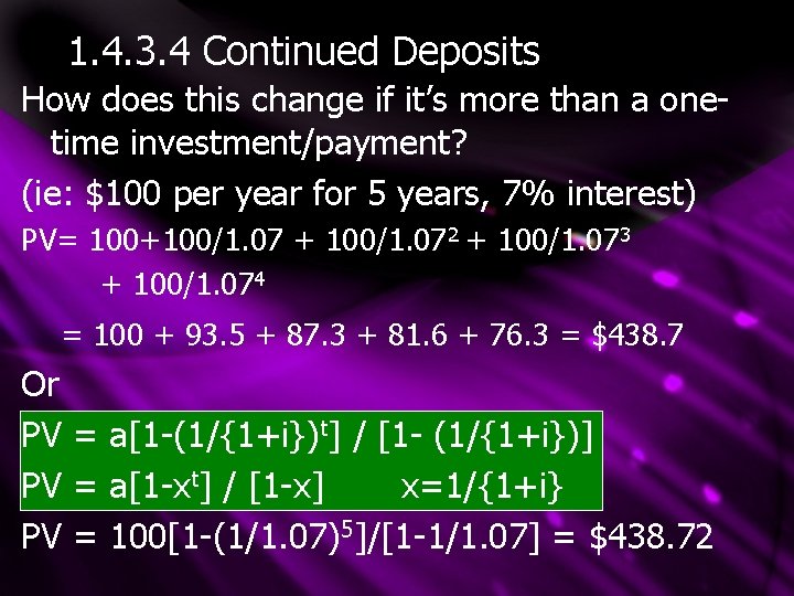
1. 4. 3. 4 Continued Deposits How does this change if it’s more than a onetime investment/payment? (ie: $100 per year for 5 years, 7% interest) PV= 100+100/1. 07 + 100/1. 072 + 100/1. 073 + 100/1. 074 = 100 + 93. 5 + 87. 3 + 81. 6 + 76. 3 = $438. 7 Or PV = a[1 -(1/{1+i})t] / [1 - (1/{1+i})] PV = a[1 -xt] / [1 -x] x=1/{1+i} PV = 100[1 -(1/1. 07)5]/[1 -1/1. 07] = $438. 72

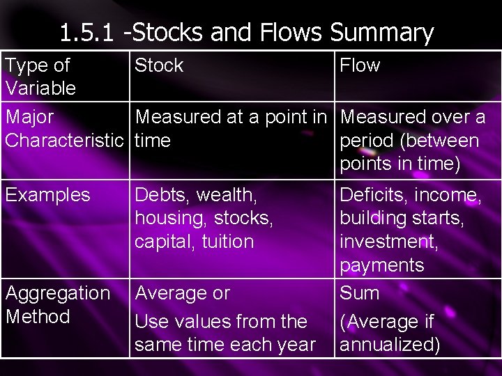
1. 5. 1 -Stocks and Flows Summary Type of Stock Flow Variable Major Measured at a point in Measured over a Characteristic time period (between points in time) Examples Debts, wealth, housing, stocks, capital, tuition Aggregation Method Average or Use values from the same time each year Deficits, income, building starts, investment, payments Sum (Average if annualized)

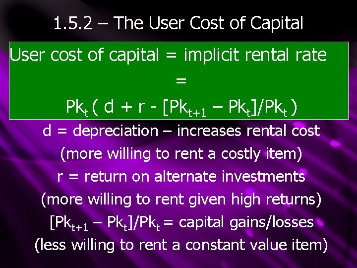
1. 5. 2 – The User Cost of Capital User cost of capital = implicit rental rate = Pkt ( d + r - [Pkt+1 – Pkt]/Pkt ) d = depreciation – increases rental cost (more willing to rent a costly item) r = return on alternate investments (more willing to rent given high returns) [Pkt+1 – Pkt]/Pkt = capital gains/losses (less willing to rent a constant value item)

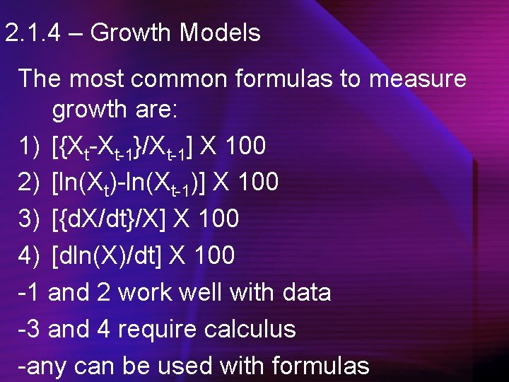
2. 1. 4 – Growth Models The most common formulas to measure growth are: 1) [{Xt-Xt-1}/Xt-1] X 100 2) [ln(Xt)-ln(Xt-1)] X 100 3) [{d. X/dt}/X] X 100 4) [dln(X)/dt] X 100 -1 and 2 work well with data -3 and 4 require calculus -any can be used with formulas

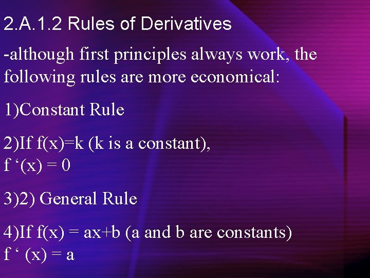
2. A. 1. 2 Rules of Derivatives -although first principles always work, the following rules are more economical: 1)Constant Rule 2)If f(x)=k (k is a constant), f ‘(x) = 0 3)2) General Rule 4)If f(x) = ax+b (a and b are constants) f ‘ (x) = a

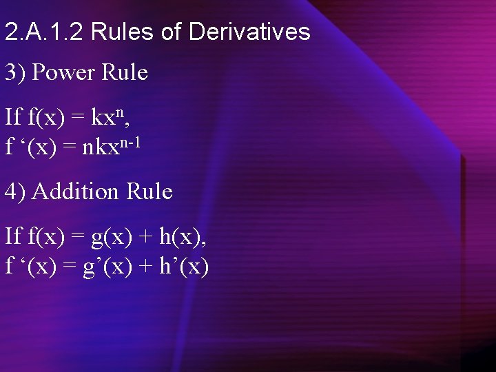
2. A. 1. 2 Rules of Derivatives 3) Power Rule If f(x) = kxn, f ‘(x) = nkxn-1 4) Addition Rule If f(x) = g(x) + h(x), f ‘(x) = g’(x) + h’(x)

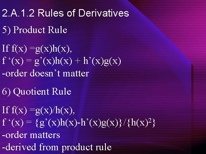
2. A. 1. 2 Rules of Derivatives 5) Product Rule If f(x) =g(x)h(x), f ‘(x) = g’(x)h(x) + h’(x)g(x) -order doesn’t matter 6) Quotient Rule If f(x) =g(x)/h(x), f ‘(x) = {g’(x)h(x)-h’(x)g(x)}/{h(x)2} -order matters -derived from product rule

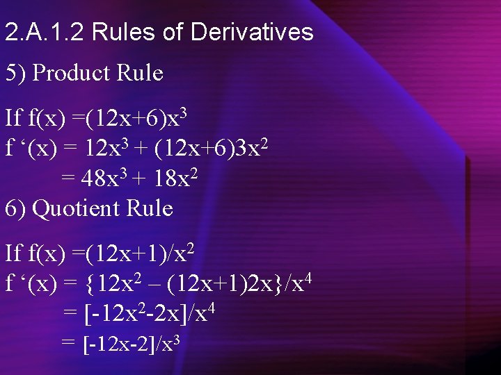
2. A. 1. 2 Rules of Derivatives 5) Product Rule If f(x) =(12 x+6)x 3 f ‘(x) = 12 x 3 + (12 x+6)3 x 2 = 48 x 3 + 18 x 2 6) Quotient Rule If f(x) =(12 x+1)/x 2 f ‘(x) = {12 x 2 – (12 x+1)2 x}/x 4 = [-12 x 2 -2 x]/x 4 = [-12 x-2]/x 3

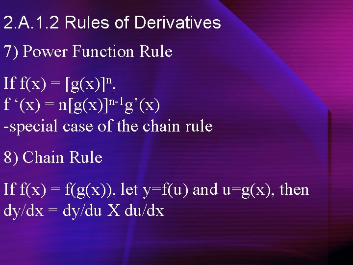
2. A. 1. 2 Rules of Derivatives 7) Power Function Rule If f(x) = [g(x)]n, f ‘(x) = n[g(x)]n-1 g’(x) -special case of the chain rule 8) Chain Rule If f(x) = f(g(x)), let y=f(u) and u=g(x), then dy/dx = dy/du X du/dx

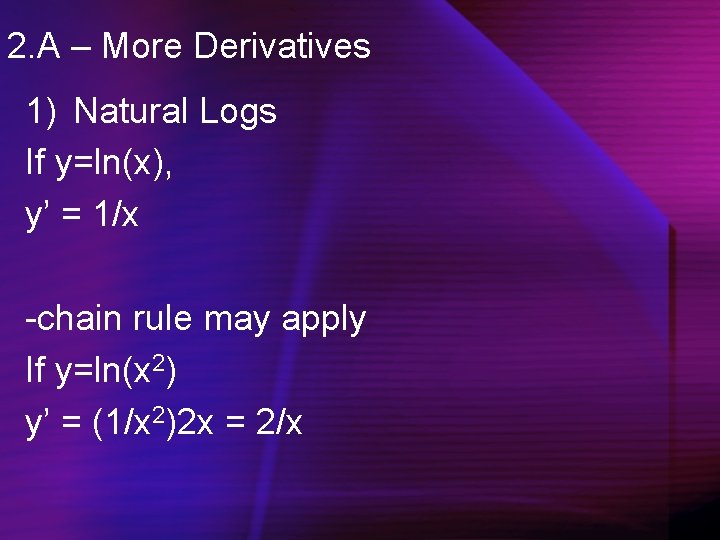
2. A – More Derivatives 1) Natural Logs If y=ln(x), y’ = 1/x -chain rule may apply If y=ln(x 2) y’ = (1/x 2)2 x = 2/x

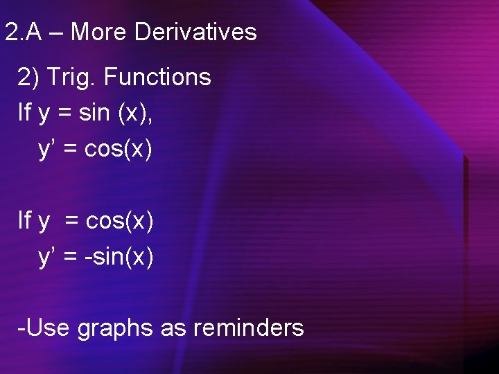
2. A – More Derivatives 2) Trig. Functions If y = sin (x), y’ = cos(x) If y = cos(x) y’ = -sin(x) -Use graphs as reminders

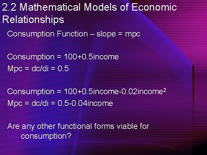
2. 2 Mathematical Models of Economic Relationships Consumption Function – slope = mpc Consumption = 100+0. 5 income Mpc = dc/di = 0. 5 Consumption = 100+0. 5 income-0. 02 income 2 Mpc = dc/di = 0. 5 -0. 04 income Are any other functional forms viable for consumption?

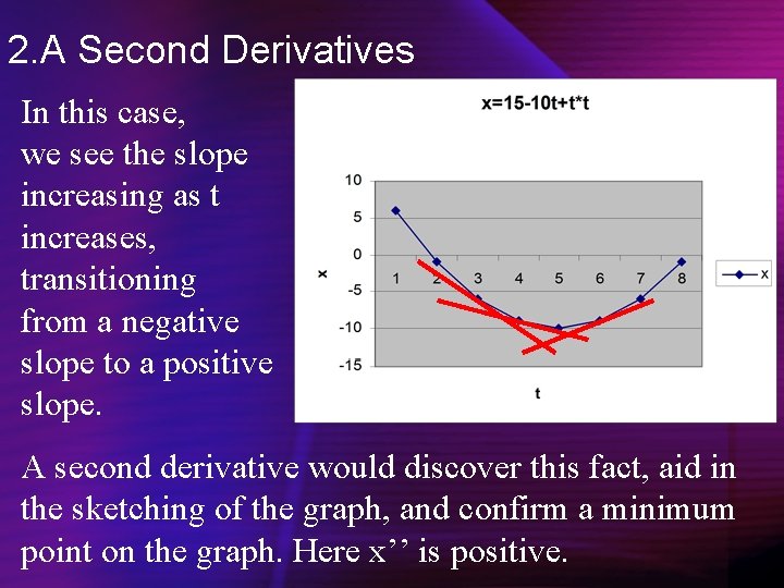
2. A Second Derivatives In this case, we see the slope increasing as t increases, transitioning from a negative slope to a positive slope. A second derivative would discover this fact, aid in the sketching of the graph, and confirm a minimum point on the graph. Here x’’ is positive.

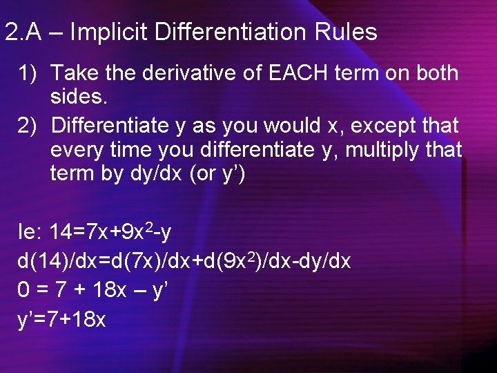
2. A – Implicit Differentiation Rules 1) Take the derivative of EACH term on both sides. 2) Differentiate y as you would x, except that every time you differentiate y, multiply that term by dy/dx (or y’) Ie: 14=7 x+9 x 2 -y d(14)/dx=d(7 x)/dx+d(9 x 2)/dx-dy/dx 0 = 7 + 18 x – y’ y’=7+18 x

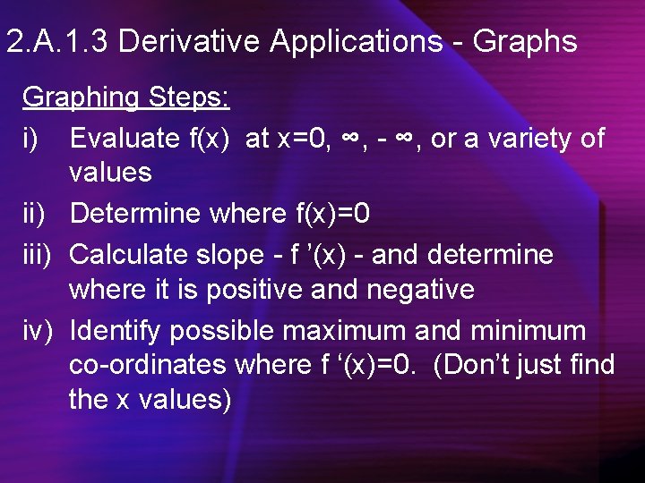
2. A. 1. 3 Derivative Applications - Graphs Graphing Steps: i) Evaluate f(x) at x=0, ∞, - ∞, or a variety of values ii) Determine where f(x)=0 iii) Calculate slope - f ’(x) - and determine where it is positive and negative iv) Identify possible maximum and minimum co-ordinates where f ‘(x)=0. (Don’t just find the x values)

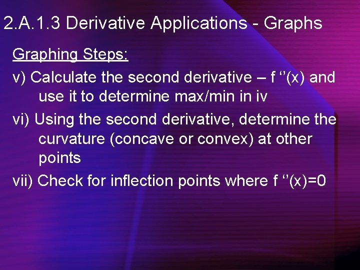
2. A. 1. 3 Derivative Applications - Graphs Graphing Steps: v) Calculate the second derivative – f ‘’(x) and use it to determine max/min in iv vi) Using the second derivative, determine the curvature (concave or convex) at other points vii) Check for inflection points where f ‘’(x)=0

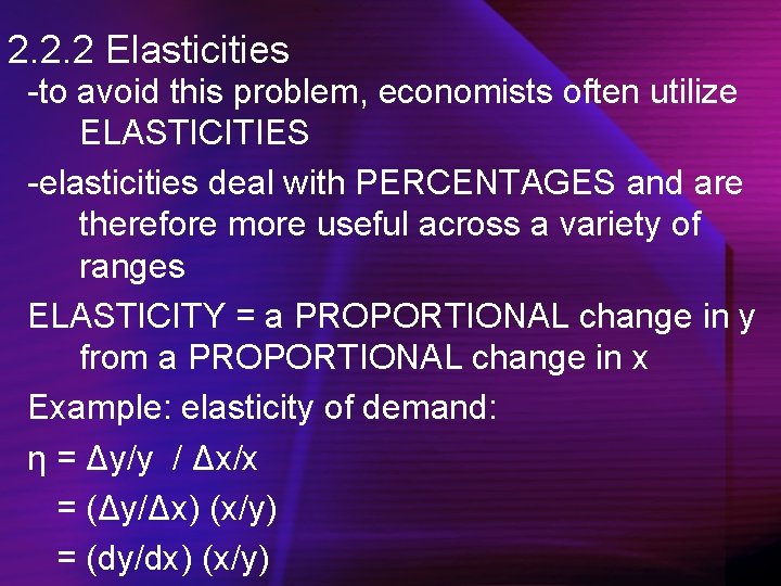
2. 2. 2 Elasticities -to avoid this problem, economists often utilize ELASTICITIES -elasticities deal with PERCENTAGES and are therefore more useful across a variety of ranges ELASTICITY = a PROPORTIONAL change in y from a PROPORTIONAL change in x Example: elasticity of demand: η = Δy/y / Δx/x = (Δy/Δx) (x/y) = (dy/dx) (x/y)

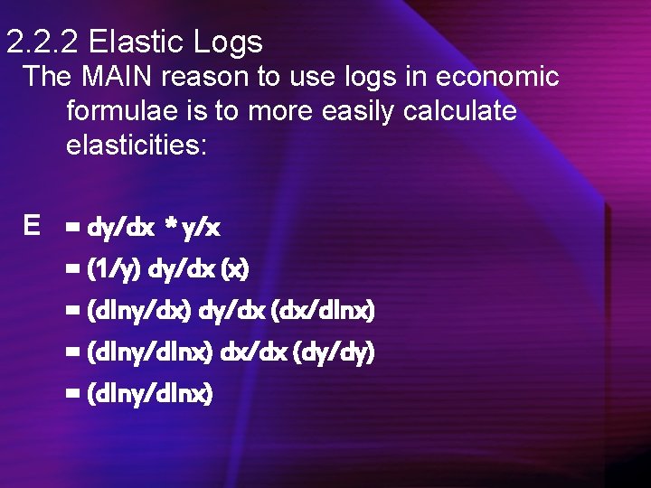
2. 2. 2 Elastic Logs The MAIN reason to use logs in economic formulae is to more easily calculate elasticities: E = dy/dx * y/x = (1/y) dy/dx (x) = (dlny/dx) dy/dx (dx/dlnx) = (dlny/dlnx) dx/dx (dy/dy) = (dlny/dlnx)

2. 3 Interpreting Parameters Unfortunately for economists, our employers are not awed and amazed by elegant equations – they want to know what the elegant equations mean. Intercepts, slopes, curvature and elasticity are thus far tools to explain models. Parameter explanation is what employers want.

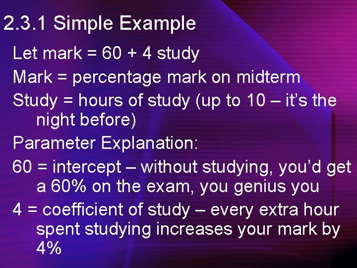
2. 3. 1 Simple Example Let mark = 60 + 4 study Mark = percentage mark on midterm Study = hours of study (up to 10 – it’s the night before) Parameter Explanation: 60 = intercept – without studying, you’d get a 60% on the exam, you genius you 4 = coefficient of study – every extra hour spent studying increases your mark by 4%

2. A The Partial Derivative It is often impossible to analyze all various movements of explanatory variables and their impact on the dependent variable. Instead, we analyze one variable’s impact, assuming ALL OTHER VARIABLES REMAIN CONSTANT We do this through the partial derivative.

2. 4 The error term Although economists try to model real behavior, their attempts are not always 100% accurate, for a variety of reasons: 1) 2) 3) 4) Excluded variables Random events (shocks) Error in data collection Economist stayed up late watching the hockey game (which could cause the above)

2. A Optimizing There are three steps for optimization: 1) Find where f’(x)=0. This is your FIRST ORDER CONDITION (FOC) and gives potential maxima/minima. 2) Evaluate f’’(x) at your potential maxima/minima. This is your SECOND ORDER CONDITION (SOC) and determines maxima/minima/inflection point status 3) Obtain the co-ordinates of your maxima/minima

2. A Local vrs. Global Thus far, our efforts have revealed LOCAL maxima and minima. It is possible, however, that such these values are not the maximum or minimum possible. These values may not be the best policy decision for a government, individual, or firm.

3. 2 Probabilities • Probabilities are assigned to the various outcomes of random variables Terminology: Sample Space – set of all possible outcomes from a random experiment -ie S = {2, 3, 4, 5, 6, 7, 8, 9, 10, 11, 12} -ie E = {Pass exam, Fail horribly} Event – a subset of the sample space -ie B = {3, 6, 9, 12} ε S -ie F = {Fail exam, Fail horribly} ε E

3. 2 Probabilities Terminology: Mutually Exclusive Events – Two events are mutually exclusive if they cannot occur at the same time -ie: rolling both a 3 and an 11; being both dead and alive; having both a son and a daughter (and only one child) Exhaustive Events – cover all possible outcomes -ie: a dice roll must lie within S ε [2, 12] -ie: a person is either married or not married

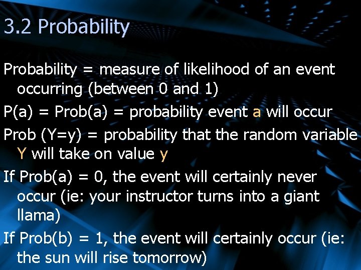
3. 2 Probability = measure of likelihood of an event occurring (between 0 and 1) P(a) = Prob(a) = probability event a will occur Prob (Y=y) = probability that the random variable Y will take on value y If Prob(a) = 0, the event will certainly never occur (ie: your instructor turns into a giant llama) If Prob(b) = 1, the event will certainly occur (ie: the sun will rise tomorrow)

3. 2 Probability Rules 1) P(a) must be greater than or equal to 0 and less than or equal to 1 : 0≤P(a) ≤ 1 2) If a set of events {A, B, C} are exhaustive, then P(A or B or C) = 1 Ie: Prob. a die roll is between 2 and 12 3) If a set of events {A, B, C} are mutually exclusive, then P(A or B or C)=P(A)+P(B)+P(C) Ie: Prob. of drawing a heart or spade

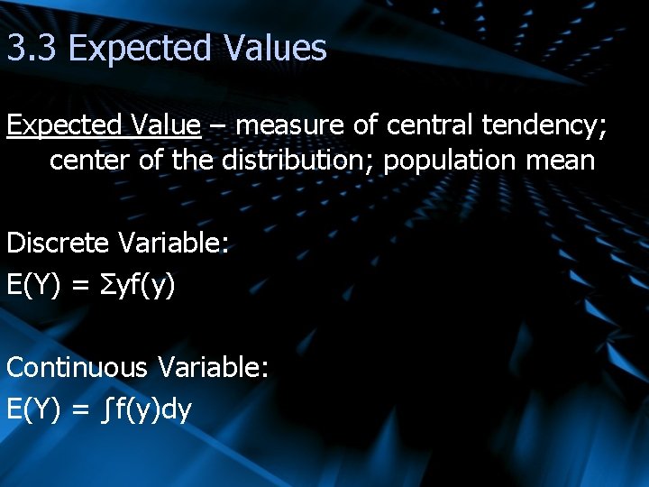
3. 3 Expected Values Expected Value – measure of central tendency; center of the distribution; population mean Discrete Variable: E(Y) = Σyf(y) Continuous Variable: E(Y) = ∫f(y)dy

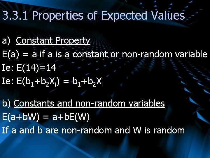
3. 3. 1 Properties of Expected Values a) Constant Property E(a) = a if a is a constant or non-random variable Ie: E(14)=14 Ie: E(b 1+b 2 Xi) = b 1+b 2 Xi b) Constants and non-random variables E(a+b. W) = a+b. E(W) If a and b are non-random and W is random

3. 4 Variance Formula Var(Y) = E(Y-E(Y))2 = E(Y 2) – [E(Y)]2 Discrete Random Variable: Var(Y) = Σ(y-E(Y))2 f(y) Continuous Random Variable: Var(Y) = ∫(y-E(Y))2 f(y)dy

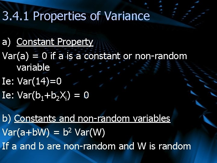
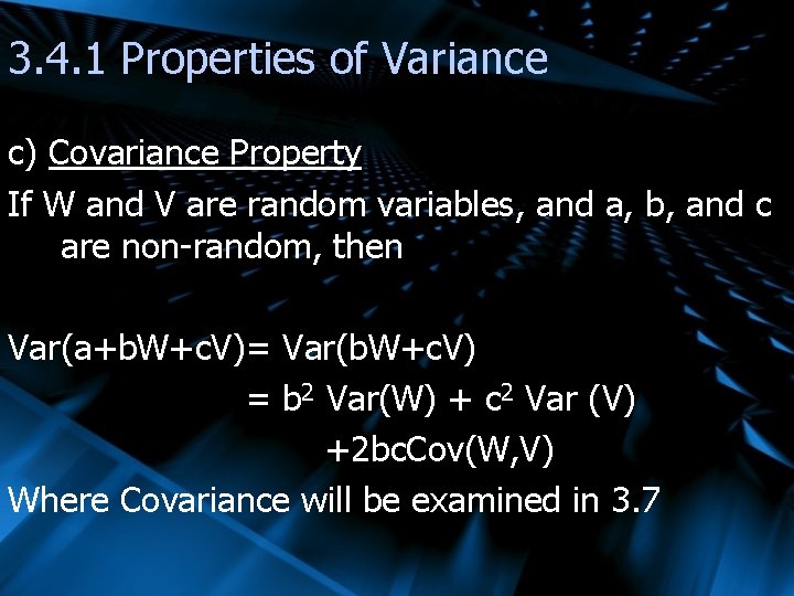
3. 4. 1 Properties of Variance a) Constant Property Var(a) = 0 if a is a constant or non-random variable Ie: Var(14)=0 Ie: Var(b 1+b 2 Xi) = 0 b) Constants and non-random variables Var(a+b. W) = b 2 Var(W) If a and b are non-random and W is random

3. 4. 1 Properties of Variance c) Covariance Property If W and V are random variables, and a, b, and c are non-random, then Var(a+b. W+c. V)= Var(b. W+c. V) = b 2 Var(W) + c 2 Var (V) +2 bc. Cov(W, V) Where Covariance will be examined in 3. 7

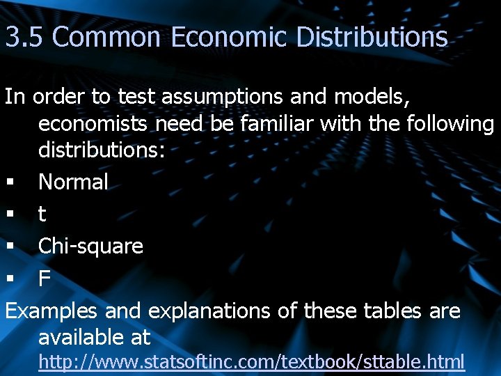
3. 5 Common Economic Distributions In order to test assumptions and models, economists need be familiar with the following distributions: § Normal § t § Chi-square § F Examples and explanations of these tables are available at http: //www. statsoftinc. com/textbook/sttable. html

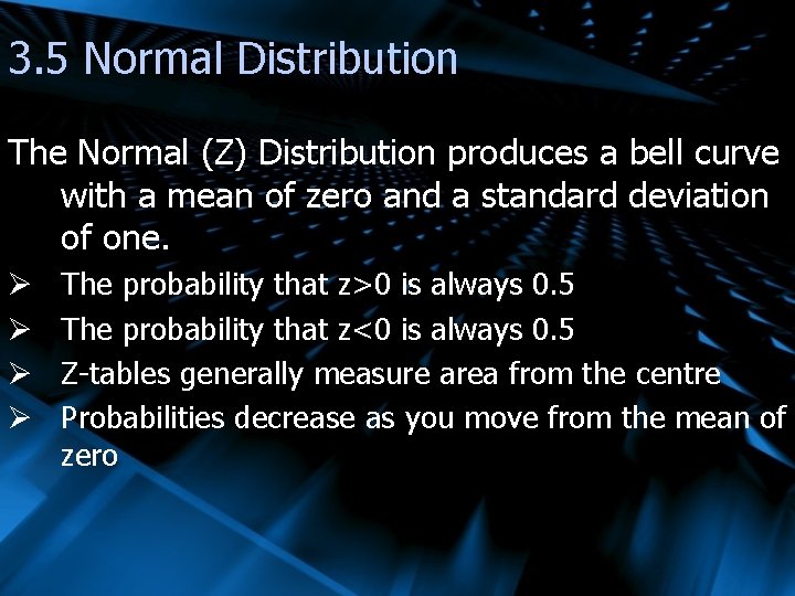
3. 5 Normal Distribution The Normal (Z) Distribution produces a bell curve with a mean of zero and a standard deviation of one. Ø Ø The probability that z>0 is always 0. 5 The probability that z<0 is always 0. 5 Z-tables generally measure area from the centre Probabilities decrease as you move from the mean of zero

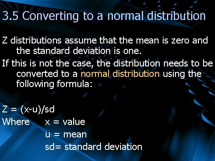
3. 5 Converting to a normal distribution Z distributions assume that the mean is zero and the standard deviation is one. If this is not the case, the distribution needs to be converted to a normal distribution using the following formula: Z = (x-u)/sd Where x = value u = mean sd= standard deviation

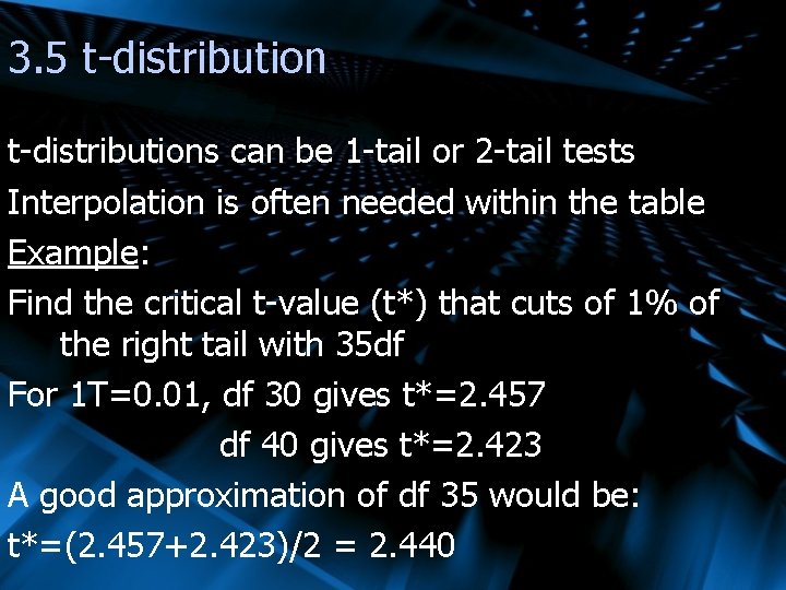
3. 5 t-distributions can be 1 -tail or 2 -tail tests Interpolation is often needed within the table Example: Find the critical t-value (t*) that cuts of 1% of the right tail with 35 df For 1 T=0. 01, df 30 gives t*=2. 457 df 40 gives t*=2. 423 A good approximation of df 35 would be: t*=(2. 457+2. 423)/2 = 2. 440

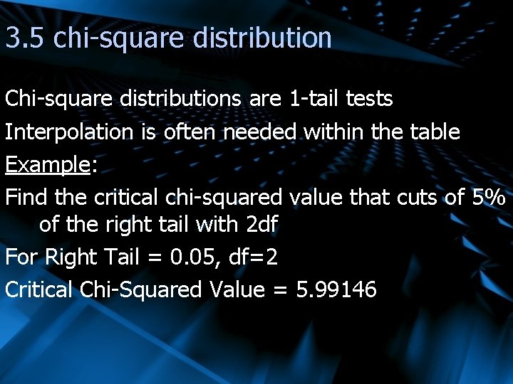
3. 5 chi-square distribution Chi-square distributions are 1 -tail tests Interpolation is often needed within the table Example: Find the critical chi-squared value that cuts of 5% of the right tail with 2 df For Right Tail = 0. 05, df=2 Critical Chi-Squared Value = 5. 99146

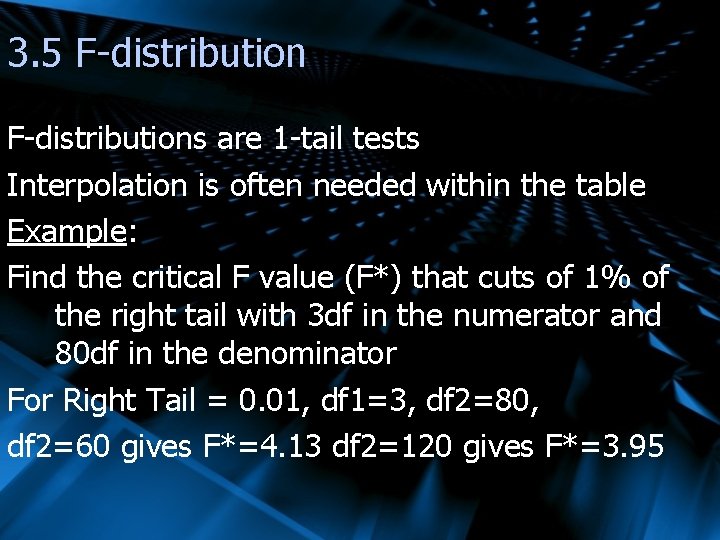
3. 5 F-distributions are 1 -tail tests Interpolation is often needed within the table Example: Find the critical F value (F*) that cuts of 1% of the right tail with 3 df in the numerator and 80 df in the denominator For Right Tail = 0. 01, df 1=3, df 2=80, df 2=60 gives F*=4. 13 df 2=120 gives F*=3. 95

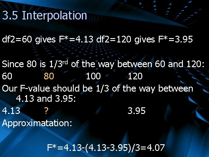
3. 5 Interpolation df 2=60 gives F*=4. 13 df 2=120 gives F*=3. 95 Since 80 is 1/3 rd of the way between 60 and 120: 60 80 100 120 Our F-value should be 1/3 of the way between 4. 13 and 3. 95: 4. 13 ? 3. 95 Approximatation: F*=4. 13 -(4. 13 -3. 95)/3=4. 07

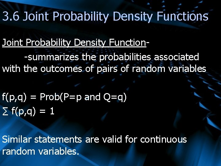
3. 6 Joint Probability Density Functions Joint Probability Density Function-summarizes the probabilities associated with the outcomes of pairs of random variables f(p, q) = Prob(P=p and Q=q) ∑ f(p, q) = 1 Similar statements are valid for continuous random variables.

3. 6 Joint and Marginal Pdf’s Marginal (individual) pdf’s can be determined from joint pdf’s. Simply add all of the joint probabilities containing the desired outcome of one of the variables. Ie: f(Y=7)=∑f(Y=7, Z=zi) Probability of Y=7 = sum of ALL joint probabilities where Y=7

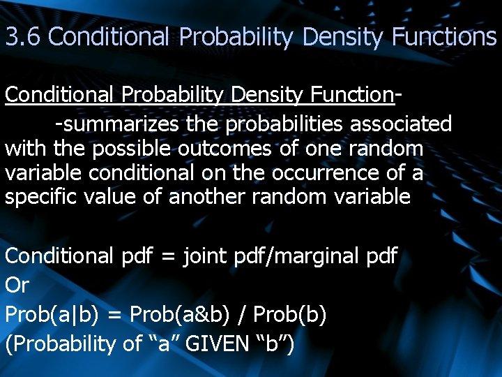
3. 6 Conditional Probability Density Functions Conditional Probability Density Function-summarizes the probabilities associated with the possible outcomes of one random variable conditional on the occurrence of a specific value of another random variable Conditional pdf = joint pdf/marginal pdf Or Prob(a|b) = Prob(a&b) / Prob(b) (Probability of “a” GIVEN “b”)

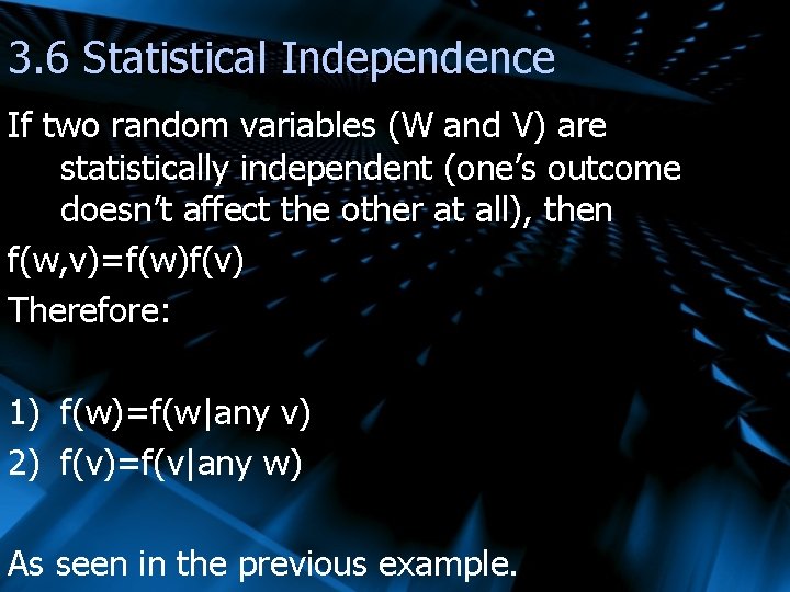
3. 6 Statistical Independence If two random variables (W and V) are statistically independent (one’s outcome doesn’t affect the other at all), then f(w, v)=f(w)f(v) Therefore: 1) f(w)=f(w|any v) 2) f(v)=f(v|any w) As seen in the previous example.

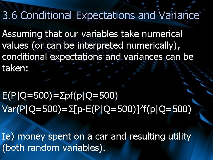
3. 6 Conditional Expectations and Variance Assuming that our variables take numerical values (or can be interpreted numerically), conditional expectations and variances can be taken: E(P|Q=500)=Σpf(p|Q=500) Var(P|Q=500)=Σ[p-E(P|Q=500)]2 f(p|Q=500) Ie) money spent on a car and resulting utility (both random variables).

3. 7 Discrete and Continuous Covariance Discrete Random Variable: Continuous Random Variable:

3. 7 Correlation:

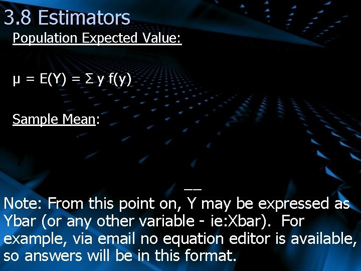
3. 8 Estimators Population Expected Value: μ = E(Y) = Σ y f(y) Sample Mean: __ Note: From this point on, Y may be expressed as Ybar (or any other variable - ie: Xbar). For example, via email no equation editor is available, so answers will be in this format.

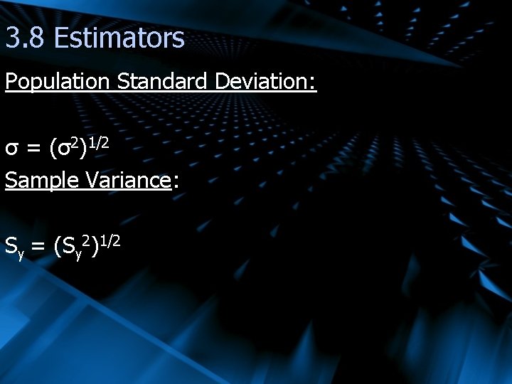
3. 8 Estimators Population Variance: σ2 = Var(Y) = Σ [y-E(y)] f(y) Sample Variance:

3. 8 Estimators Population Standard Deviation: σ = (σ2)1/2 Sample Variance: Sy = (Sy 2)1/2

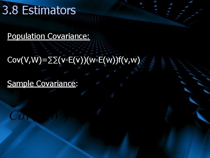
3. 8 Estimators Population Covariance: Cov(V, W)=∑∑(v-E(v))(w-E(w))f(v, w) Sample Covariance:

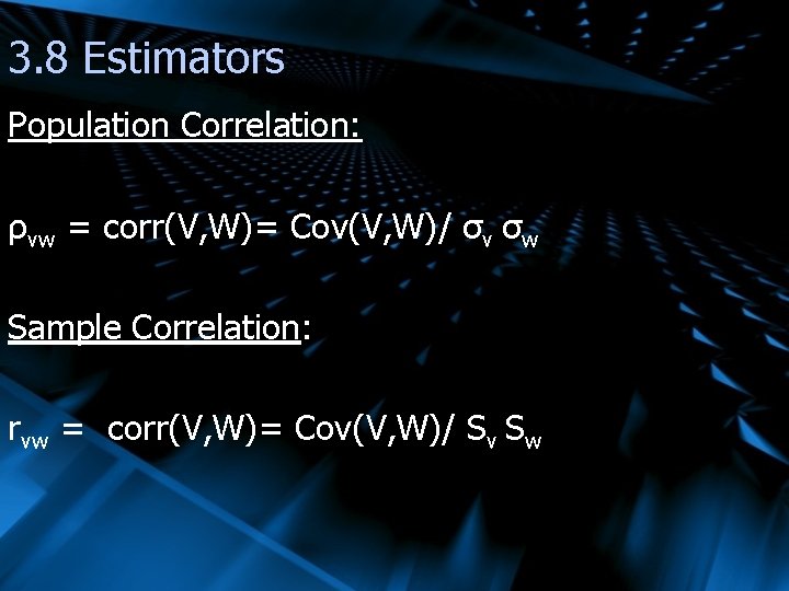
3. 8 Estimators Population Correlation: ρvw = corr(V, W)= Cov(V, W)/ σv σw Sample Correlation: rvw = corr(V, W)= Cov(V, W)/ Sv Sw

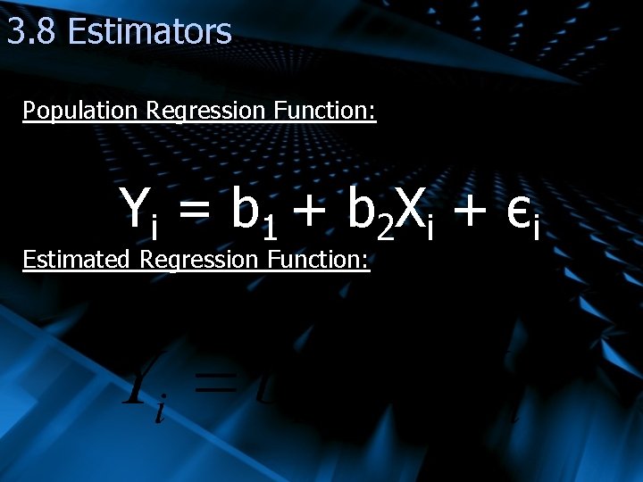
3. 8 Estimators Population Regression Function: Yi = b 1 + b 2 X i + єi Estimated Regression Function:

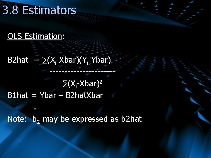
3. 8 Estimators OLS Estimation: B 2 hat = ∑(Xi-Xbar)(Yi-Ybar) -----------∑(Xi-Xbar)2 B 1 hat = Ybar – B 2 hat. Xbar ^ Note: b 2 may be expressed as b 2 hat

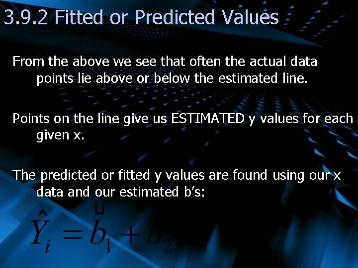
3. 9. 2 Fitted or Predicted Values From the above we see that often the actual data points lie above or below the estimated line. Points on the line give us ESTIMATED y values for each given x. The predicted or fitted y values are found using our x data and our estimated b’s:

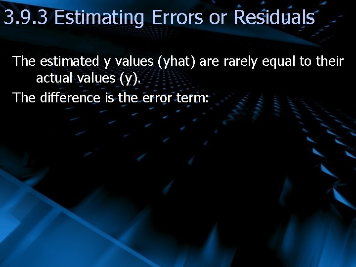
3. 9. 3 Estimating Errors or Residuals The estimated y values (yhat) are rarely equal to their actual values (y). The difference is the error term:

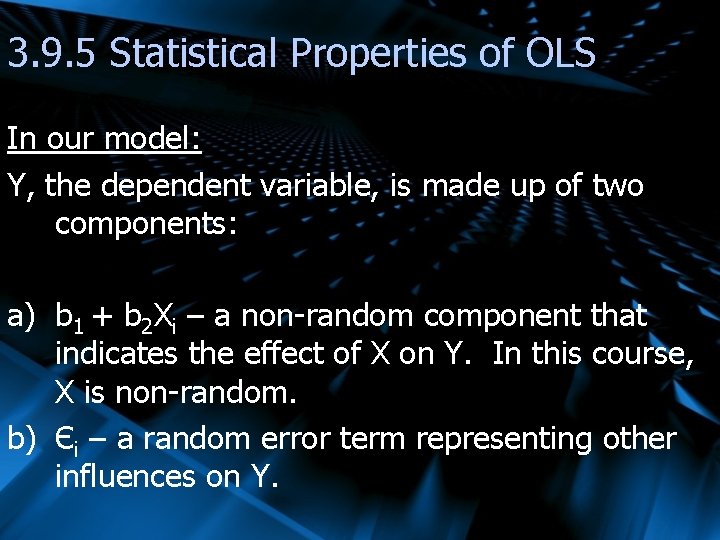
3. 9. 5 Statistical Properties of OLS In our model: Y, the dependent variable, is made up of two components: a) b 1 + b 2 Xi – a non-random component that indicates the effect of X on Y. In this course, X is non-random. b) Єi – a random error term representing other influences on Y.

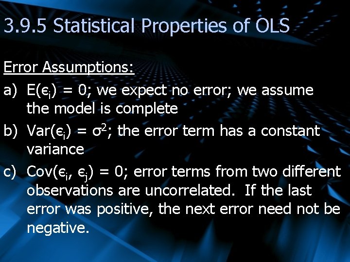
3. 9. 5 Statistical Properties of OLS Error Assumptions: a) E(єi) = 0; we expect no error; we assume the model is complete b) Var(єi) = σ2; the error term has a constant variance c) Cov(єi, єj) = 0; error terms from two different observations are uncorrelated. If the last error was positive, the next error need not be negative.

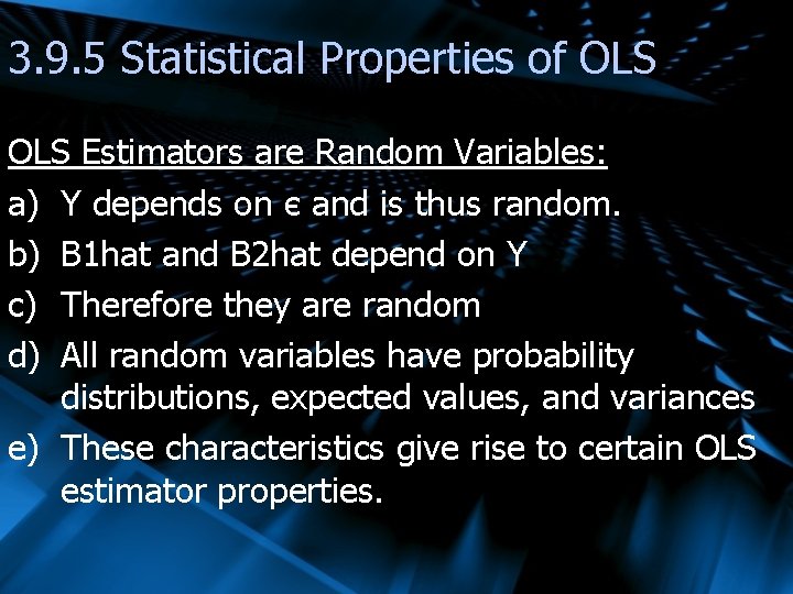
3. 9. 5 Statistical Properties of OLS Estimators are Random Variables: a) Y depends on є and is thus random. b) B 1 hat and B 2 hat depend on Y c) Therefore they are random d) All random variables have probability distributions, expected values, and variances e) These characteristics give rise to certain OLS estimator properties.

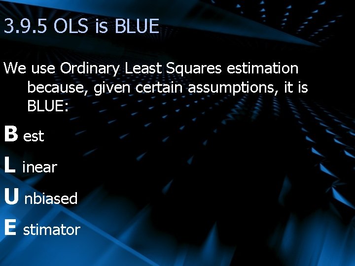
3. 9. 5 OLS is BLUE We use Ordinary Least Squares estimation because, given certain assumptions, it is BLUE: B est L inear U nbiased E stimator

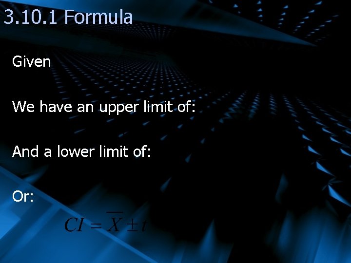
3. 10. 1 Formula Given We have an upper limit of: And a lower limit of: Or:

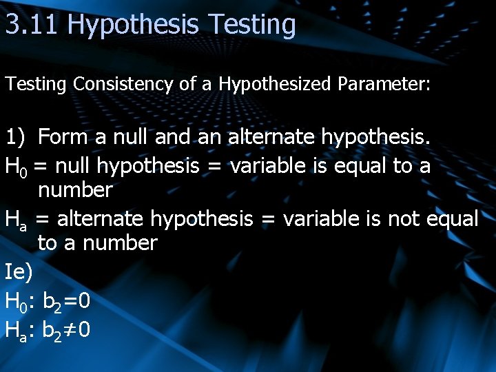
3. 11 Hypothesis Testing Consistency of a Hypothesized Parameter: 1) Form a null and an alternate hypothesis. H 0 = null hypothesis = variable is equal to a number Ha = alternate hypothesis = variable is not equal to a number Ie) H 0: b 2=0 Ha: b 2≠ 0

3. 11 Hypothesis Testing Consistency of a Hypothesized Parameter: 2) Collect appropriate sample data 3) Select an acceptable probability (α) of rejecting a null hypothesis when it is true -Type one error -Lower α, more unlikely to find a sample that rejects the null hypothesis - α is often 10%, 5%, or 1%

3. 11 Hypothesis Testing Consistency of a Hypothesized Parameter: 4) Construct an appropriate test statistic -ensure the test statistic can be calculated from the sample data -ensure its distribution is appropriate to that being tested (ie: t-statistic for test for mean)

3. 11 Hypothesis Testing Consistency of a Hypothesized Parameter: 5) Establish (do not) reject regions -Construct bell curve -Tails are Reject H 0 regions -Centre is Do not Reject H 0 regions

3. 11 Hypothesis Testing Consistency of a Hypothesized Parameter: 6) Compare the test statistic to the critical statistic -If the test statistic lies in the tails, reject -If the test statistic doesn’t lie in the tails, do not reject -Never Accept 7) Interpret Results

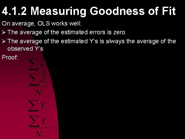
4. 1. 2 Measuring Goodness of Fit On average, OLS works well: Ø The average of the estimated errors is zero Ø The average of the estimated Y’s is always the average of the observed Y’s Proof:

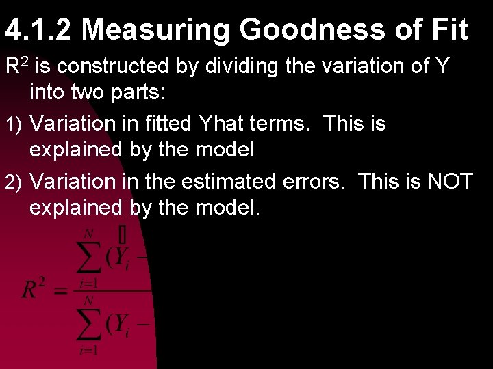
4. 1. 2 Measuring Goodness of Fit R 2 is constructed by dividing the variation of Y into two parts: 1) Variation in fitted Yhat terms. This is explained by the model 2) Variation in the estimated errors. This is NOT explained by the model.

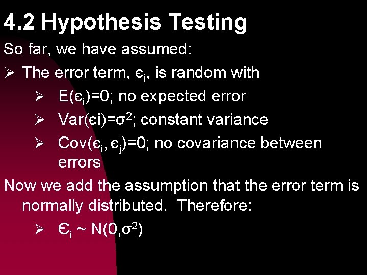
4. 2 Hypothesis Testing So far, we have assumed: Ø The error term, єi, is random with Ø E(єi)=0; no expected error Ø Var(єi)=σ2; constant variance Ø Cov(єi, єj)=0; no covariance between errors Now we add the assumption that the error term is normally distributed. Therefore: Ø Єi ~ N(0, σ2)

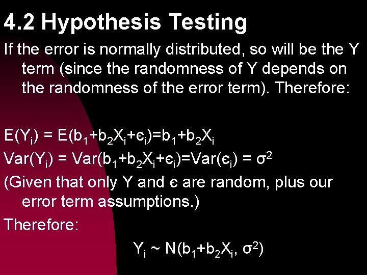
4. 2 Hypothesis Testing If the error is normally distributed, so will be the Y term (since the randomness of Y depends on the randomness of the error term). Therefore: E(Yi) = E(b 1+b 2 Xi+єi)=b 1+b 2 Xi Var(Yi) = Var(b 1+b 2 Xi+єi)=Var(єi) = σ2 (Given that only Y and є are random, plus our error term assumptions. ) Therefore: Yi ~ N(b 1+b 2 Xi, σ2)

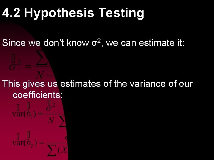
4. 2 Hypothesis Testing Since we don’t know σ2, we can estimate it: This gives us estimates of the variance of our coefficients:

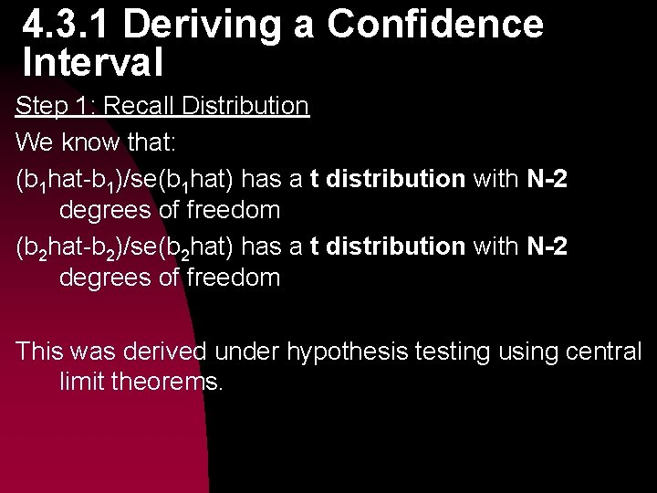
4. 3. 1 Deriving a Confidence Interval Step 1: Recall Distribution We know that: (b 1 hat-b 1)/se(b 1 hat) has a t distribution with N-2 degrees of freedom (b 2 hat-b 2)/se(b 2 hat) has a t distribution with N-2 degrees of freedom This was derived under hypothesis testing using central limit theorems.

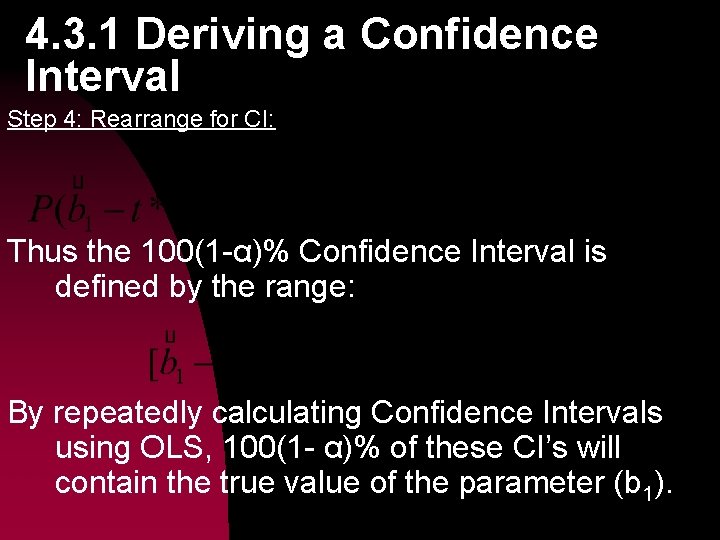
4. 3. 1 Deriving a Confidence Interval Step 4: Rearrange for CI: Thus the 100(1 -α)% Confidence Interval is defined by the range: By repeatedly calculating Confidence Intervals using OLS, 100(1 - α)% of these CI’s will contain the true value of the parameter (b 1).

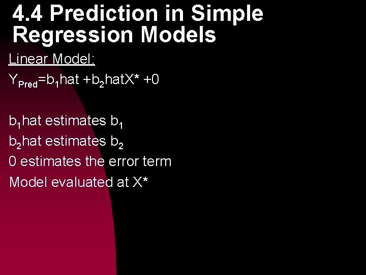
4. 4 Prediction in Simple Regression Models Linear Model: YPred=b 1 hat +b 2 hat. X* +0 b 1 hat estimates b 1 b 2 hat estimates b 2 0 estimates the error term Model evaluated at X*

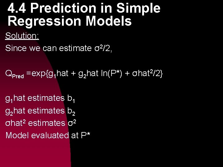
4. 4 Prediction in Simple Regression Models Solution: Since we can estimate σ2/2, QPred =exp{g 1 hat + g 2 hat ln(P*) + σhat 2/2} g 1 hat estimates b 1 g 2 hat estimates b 2 σhat 2 estimates σ2 Model evaluated at P*