Structural Equation Modelling Professor Luiz Moutinho Structural Equation

Structural Equation Modelling Professor Luiz Moutinho

Structural Equation Modelling Overview Structural equation modelling (SEM) grows out of and serves purposes similar to multiple regression, but in a more powerful way which takes into account the modelling of interactions, nonlinearities, correlated independents, measurement error, correlated error items, multiple latent independents each measured by multiple indicators, and one or more latent dependents also each with multiple indicators. SEM may be used as a more powerful alternative to multiple regression, path analysis, factor analysis, time series analysis, and analysis of covariance. SEM is an extension of the General Linear Model (GLM)

Structural Equation Modelling Advantages of SEM compared to multiple regression include more flexible assumptions (particularly allowing interpretation even in the face of multicollinearity), use of confirmatory factor analysis to reduce measurement error by having multiple indicators per latent variable, the attraction of SEM’s graphical modelling interface, the desirability of testing models overall rather than coefficients individually, the ability to test models with multiple dependents, the ability to model mediating variables, the ability to model error terms, the ability to test coefficients across multiple between-subjects groups, and ability to handle difficult data (time services with autocorrelated error, non-normal data, incomplete data).

Structural Equation Modelling SEM is usually viewed as a confirmatory rather than exploratory procedure, using one of three approaches: 1. Strictly confirmatory approach: A model is tested using SEM goodness-of-fit tests to determine if the pattern of variances and covariances in the data is consistent with a structural (path) model specified by the researcher. However as other unexamined models may fit the data as well or better, an accepted model is only a notdisconfirmed model.

Structural Equation Modelling 2. 3. Alternative models approach: One may test two or more causal models to determine which has the best fit. There are many goodness-of-fit measures, reflecting different considerations, and usually three or four are reported by the researcher. Although desirable in principle, this AM approach runs into the real-world problem that in most specific research topic areas, the researcher does not find in the literature two well-developed alternative models to test. Model development approach: In practice, much SEM research combines confirmatory and exploratory purposes: a model is tested using SEM procedures, found to be deficient, and an alternative model is then tested based on changes suggested by SEM modification indexes. This is the most common approach found in the literature. The problem with the model development approach is that models confirmed in this manner are post-hoc ones which may not be stable (may not fit new data, having been created based on the uniqueness of an initial dataset). Researchers may attempt to overcome this problem by using a cross-validation strategy under which the model is developed using a calibration data sample and then confirmed using an independent validation sample.

Structural Equation Modelling Regardless of approach, SEM cannot itself draw casual arrows in models or resolve causal ambiguities. SEM is a family of statistical techniques which incorporates and integrates path analysis and factor analysis. In fact, use of SEM software for a model in which each variable has only one indicator is a type of path analysis. Use of SEM software for a model in which each variable has multiple indicators but there are no direct effects (arrows) connecting the variables is a type of factor analysis. Synonyms for SEM are covariance structure analysis, covariance structure modelling, and analysis of covariance structures. See also Partial least squares regression, which is sometimes used to predict one set of response variables from a set of independent variables which can also generate path coefficients for a SEM-type model.

Structural Equation Modelling Key Concepts and Terms • • • The structural equation modelling process centres around two steps: validating the measurement model and fitting the structural model. The former is accomplished primarily through confirmatory factor analysis, while the latter is accomplished primarily through path analysis with latent variables. One starts by specifying a model on the basis of theory. Each variable in the model is conceptualized as a latent one, measured by the multiple indicators. Based on a large (n>100) representative sample, factor analysis (common factor analysis or principal axis factoring, not principal components analysis) is used to establish that indicators seem to measure the corresponding latent variables, represented by the factors. Two or more alternative models (one of which may be the null model) are then compared in terms of “model fit, ” which measures the extent to which the covariances predicted by the model correspond to the observed covariances in the data. “Modification indexes” and other coefficients may be used by the researcher to alter one or more models to improve fit.

Structural Equation Modelling Key Concepts and Terms • • • LISREL, AMOS, and EQS are three popular statistical packages for doing SEM. AMOS (Analysis of MOment Structures) is a more recent package which, because of its user-friendly graphical interface, has become popular as an easier way of specifying structural models. Indicators are observed variables, sometimes called manifest variables or reference variables, such as items in a survey instrument. Latent Variables are the unobserved variables or constructs or factors which are measured by their respective indicators. Latent variables include both independent, mediating, and dependent variables. “Exogenous” variables are independents with no prior causal variable (though they may be correlated with other exogenous variables, depicted by a double-headed arrow – note two latent variables can be connected by a double-headed arrow (correlation) or a single-headed arrow (causation) but not both.

Structural Equation Modelling • • “Endogenous” variables are mediating variables (variables which are both effects of other exogenous or mediating variables, and are causes of other mediating and dependent variables), and pure dependent variables. Variables in a model may be “upstream” or “downstream” depending on whether they are being considered as causes or effects respectively. The representation of latent variables based on their relation to observed indicator variables is one of the defining characteristics of SEM. Warning: Indicator variables cannot be combined arbitrarily to form latent variables. For instance, combining gender, race, or other demographic variables to form a latent variable called “background factors” would be improper because it would not represent any single underlying continuum of meaning. The confirmatory factor analysis step in SEM is a test of the meaningfulness of latent variables and their indicators.

Structural Equation Modelling Key Concepts and Terms • • The measurement model is that part (possibly all) of a SEM model which deals with the latent variables and their indicators. A pure measurement model is a confirmatory factor analysis (CFA) model in which there is unmeasured covariance between each possible pair of latent variables, there are straight arrows from the latent variables to their respective indicators, there are straight arrows from the error and disturbance terms to their respective variables, but there are no direct effects (straight arrows) connecting the latent variables. The measurement model is evaluated like any other SEM model, using goodness of fit measures.

Structural Equation Modelling Key Concepts and Terms • • The null model. The measurement model is frequently used as the “null model, ” differences from which must be significant if a proposed structural model (the one with straight arrows connecting some latent variables) is to be investigated further. In the null model, the covariances in the covariance matrix for the latent variables are all assumed to be zero. The structural model may be contrasted with the measurement model. It is the set of exogenous and endogenous variables in the model, together with the direct effects (straight arrows) connecting them, and the disturbance terms for these variables (reflecting the effects of unmeasured variables not in the model). Confirmatory factor analysis plays an important role in structural equation modelling. CFA models in SEM are used to assess the role of measurement error in the model, to validate a multifactorial model and determine group effects on the Factors.

Structural Equation Modelling Key Concepts and Terms • Model Specification is the process by which the researcher asserts which effects are null, which are fixed to a constant (usually 1. 0), and which vary. Variable effects correspond to arrows in the model, while null effects correspond to an absence of an arrow. Model Parsimony. Adding paths will tend to increase fit. Ways to decrease model complexity are erasing direct effects (straight arrows) from one latent variable to another; erasing direct effects from multiple latent variables to the same indicator variable; and erasing unanalyzed correlations (curved double-headed arrows) between measurement error terms and between the disturbance terms of the endogenous variables.

Structural Equation Modelling Key Concepts and Terms • • Metric: In SEM, each unobserved latent variable must be assigned explicitly a metric, which is a measurement range. This is normally done by constraining one of the paths from the latent variable to one of its indicator (reference) variables, as by assigning the value of 1. 0 to this path. The indicator selected to be constrained to 1. 0 is the reference item. Typically one selects as the reference item the one which in factor analysis loads most heavily on the dimension represented by the latent variable, thereby allowing it to anchor the meaning of that dimension.

Structural Equation Modelling Key Concepts and Terms • • • Error and disturbance terms. An error term refers to the measurement error factor associated with a given indicator. Whereas regression models implicitly assume zero measurement error (that is, to the extent such error exists, regression coefficients are attenuated), error terms are explicitly modelled in SEM and as a result path coefficients modelled in SEM are unbiased by error terms, whereas regression coefficients are not. Note these measurement error terms are not to be confused with residual error terms, also called disturbance terms, which reflect the unexplained variance in the latent endogenous variable(s) due to all unmeasured causes. Uncorrelated error terms are an assumption of regression, whereas the correlation of error terms may and should be explicitly modelled in SEM. That is, in regression the researcher models variables, whereas in SEM the researcher must model error as well as the variables.

Structural Equation Modelling Key Concepts and Terms • Structural or Path coefficients are the effect sizes calculated by the model estimation program. In AMOS, these are labelled “regression weights, ” which is what they are, except that in the structural equation there will be no intercept term. 1. • Types of estimation of coefficients in SEM. Structural coefficients in SEM may be computed any of several ways. Ordinarily, one will get similar estimates by any of the methods. MLE. Maximum Likelihood Estimation (MLE) is by far the most common method. MLE makes estimates based on maximising the probability (likelihood) that the observed covariances are drawn from a population assumed to be the same as that reflected in the coefficient estimates. That is, MLE picks estimates which have the greatest chance of reproducing the observed data.

Structural Equation Modelling Key Concepts and Terms Assumptions: Unlike OLS regression estimates, MLE does not assume uncorrelated error terms and thus may be used for non-recursive as well as recursive models. Key assumptions of MLE are large samples; indicator variables with multivariate normal distribution; and continuous indicator variations (though ordinal variables are widely used in practice). If ordinal data are used, they should have at least five categories and not be strongly skewed. MLE estimates of variances, covariances, and paths to disturbance terms. Whereas MLE differs from OLS in estimating structural (path) coefficients relating variables, it uses the same method (i. e. , the observed values) as estimates for the variances and covariances if the exogenous variables. Each path from a latent endogenous variable to its disturbance term is set to 1. 0, thereby allowing SEM to estimate the variance of the disturbance item.

Structural Equation Modelling • Other estimation methods do exist. GLS (Generalized Least Squares) is the second most popular method after MLE. GLS works well for large samples (n>2500) even for non-normal data. 2. Standardized structural (path) coefficients. When researchers speak of structural or path coefficients in SEM, they normally mean standardized ones. Standardized structural coefficient estimates are based on standardized data, including correlation matrixes. Standardized estimates are used, for instance, when comparing direct effects on a given endogenous variable in a single-group study. That is, as in OLS regression, the standardized weights are used to compare the relative importance of the independent variables. The interpretation is similar to regression: if a standardized structural coefficient is 2. 0, then the latent dependent will increase by 2. 0 standard units for each unit increase in the latent independent. In AMOS, the standardized structural coefficients are labelled “standardized regression weights, ” which is what they are

Structural Equation Modelling 3. The Critical Ratio and significance of path coefficients. When the Critical Ratio (CR) is > 1. 96 for a regression weight, that path is significant at the. 05 level. The significance of the standardized and unstandardized estimates will be identical. In LISREL, the critical ratio is the z-value for each gamma in the Gamma Matrix of standardized and unstandardized path coefficient estimates for the paths linking the endogenous variables. The “z-values” for paths linking the exogenous to the endogenous variables are in the Beta Matrix. If the z-value is greater than or equal to 1. 96, then the gamma coefficient is significant at the. 05 level.

Structural Equation Modelling • • Completely standardized solution: correlation matrix of eta and KSI: In LISREL output this is the matrix of correlations of the latent independent variables. Eta is a coefficient of nonlinear correlation. Goodness of fit tests determine if the model being tested should be accepted or rejected. These overall fit tests do not establish that particular paths within the model are significant. LISREL prints 15 and AMOS prints 25 different goodness-of-fit measures, the choice of which is a matter of dispute among methodologists. There is wide disagreement in just which fit indexes to report, but one should avoid the shotgun approach of reporting all of them, which seems to imply the researcher is on a fishing expedition.

Structural Equation Modelling Warnings about interpreting fit indexes: A “good fit” is not the same as strength of relationship: one could have perfect fit when all variables in the model were totally uncorrelated, as long as the researcher does not instruct the SEM software to constrain the variances. In fact, the lower the correlations stipulated in the model, the easier it is to find “good fit. ” The stronger the correlations, the more power SEM has to detect an incorrect model.

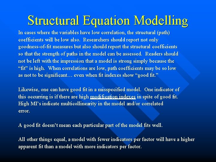
Structural Equation Modelling In cases where the variables have low correlation, the structural (path) coefficients will be low also. Researchers should report not only goodness-of-fit measures but also should report the structural coefficients so that the strength of paths in the model can be assessed. Readers should not be left with the impression that a model is strong simply because the “fit” is high. When correlations are low, path coefficients may be so low as not to be significant… even when fit indexes show “good fit. ” Likewise, one can have good fit in a misspecified model. One indicator of this occurring is if there are high modification indexes in spite of good fit. High MI’s indicate multicollinearity in the model and/or correlated error. A good fit doesn’t mean each particular part of the model fits well. All other things equal, a model with fewer indicators per factor will have a higher apparent fit than a model with more indicators per factor.

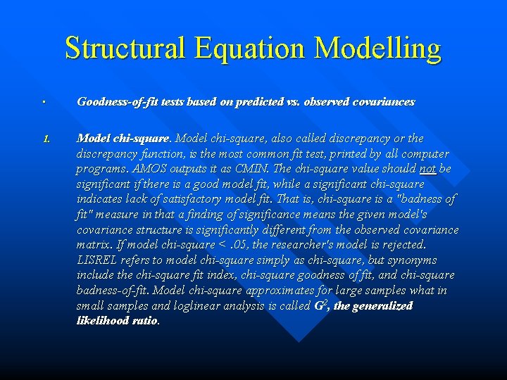
Structural Equation Modelling • Goodness-of-fit tests based on predicted vs. observed covariances 1. Model chi-square, also called discrepancy or the discrepancy function, is the most common fit test, printed by all computer programs. AMOS outputs it as CMIN. The chi-square value should not be significant if there is a good model fit, while a significant chi-square indicates lack of satisfactory model fit. That is, chi-square is a "badness of fit" measure in that a finding of significance means the given model's covariance structure is significantly different from the observed covariance matrix. If model chi-square <. 05, the researcher's model is rejected. LISREL refers to model chi-square simply as chi-square, but synonyms include the chi-square fit index, chi-square goodness of fit, and chi-square badness-of-fit. Model chi-square approximates for large samples what in small samples and loglinear analysis is called G 2, the generalized likelihood ratio.

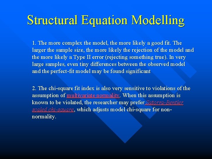
Structural Equation Modelling 1. The more complex the model, the more likely a good fit. The larger the sample size, the more likely the rejection of the model and the more likely a Type II error (rejecting something true). In very large samples, even tiny differences between the observed model and the perfect-fit model may be found significant 2. The chi-square fit index is also very sensitive to violations of the assumption of multivariate normality. When this assumption is known to be violated, the researcher may prefer Satorra-Bentler scaled chi-square, which adjusts model chi-square for nonnormality.

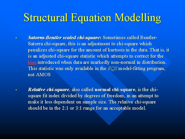
Structural Equation Modelling • Satorra-Bentler scaled chi-square: Sometimes called Bentler. Satorra chi-square, this is an adjustment to chi-square which penalizes chi-square for the amount of kurtosis in the data. That is, it is an adjusted chi-square statistic which attempts to correct for the bias introduced when data are markedly non-normal in distribution. This statistic was only available in the EQS model-fitting program, not AMOS • Relative chi-square, also called normal chi-square, is the chisquare fit index divided by degrees of freedom, in an attempt to make it less dependent on sample size. The relative chi-square should be in the 2: 1 or 3: 1 range for an acceptable model.

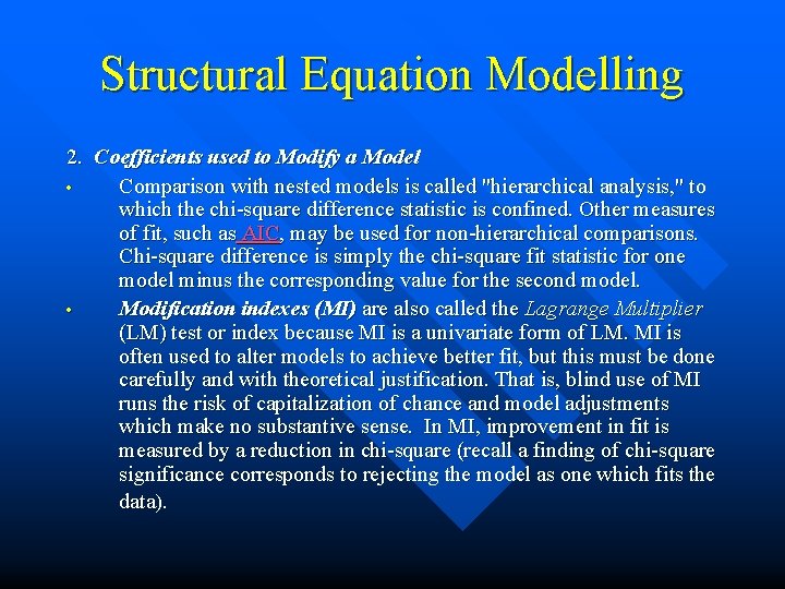
Structural Equation Modelling 2. Coefficients used to Modify a Model • Comparison with nested models is called "hierarchical analysis, " to which the chi-square difference statistic is confined. Other measures of fit, such as AIC, may be used for non-hierarchical comparisons. Chi-square difference is simply the chi-square fit statistic for one model minus the corresponding value for the second model. • Modification indexes (MI) are also called the Lagrange Multiplier (LM) test or index because MI is a univariate form of LM. MI is often used to alter models to achieve better fit, but this must be done carefully and with theoretical justification. That is, blind use of MI runs the risk of capitalization of chance and model adjustments which make no substantive sense. In MI, improvement in fit is measured by a reduction in chi-square (recall a finding of chi-square significance corresponds to rejecting the model as one which fits the data).

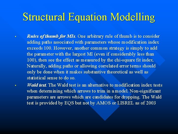
Structural Equation Modelling • • Rules of thumb for MIs. One arbitrary rule of thumb is to consider adding paths associated with parameters whose modification index exceeds 100. However, another common strategy is simply to add the parameter with the largest MI (even if considerably less than 100), then see the effect as measured by the chi-square fit index. Naturally, adding paths or allowing correlated error terms should only be done when it makes substantive theoretical as well as statistical sense to do so. Wald test. The Wald test is an alternative to modification index tests when determining which arrows to trim in a model. Non-significant parameters are arrows which are candidates for dropping. The Wald test is provided by EQS but not by AMOS or LISREL as of 2003

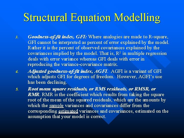
Structural Equation Modelling 3. 4. 5. Goodness-of-fit index, GFI: Where analogies are made to R-square, GFI cannot be interpreted as percent of error explained by the model. Rather it is the percent of observed covariances explained by the covariances implied by the model. That is, R 2 in multiple regression deals with error variance whereas GFI deals with error in reproducing the variance-covariance matrix. Adjusted goodness-of-fit index, AGFI is a variant of GFI which adjusts GFI for degrees of freedom. However, AGFI’s use has been declining. Root mean square residuals, or RMSR, or RMR is the coefficient which results from taking the square root of the mean of the squared residuals, which are the amounts by which the sample variances and covariances differ from the corresponding estimated variances and covariances, estimated on the assumption that your model is correct.

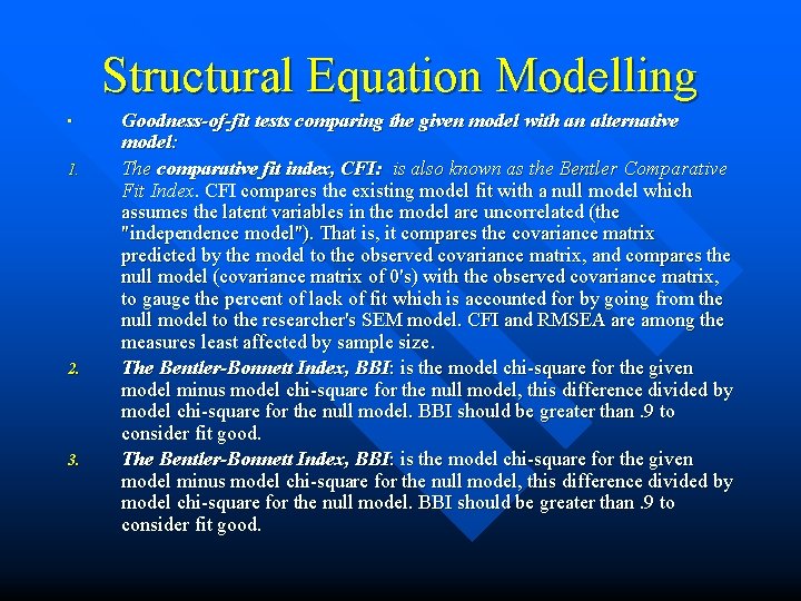
Structural Equation Modelling • 1. 2. 3. Goodness-of-fit tests comparing the given model with an alternative model: The comparative fit index, CFI: is also known as the Bentler Comparative Fit Index. CFI compares the existing model fit with a null model which assumes the latent variables in the model are uncorrelated (the "independence model"). That is, it compares the covariance matrix predicted by the model to the observed covariance matrix, and compares the null model (covariance matrix of 0's) with the observed covariance matrix, to gauge the percent of lack of fit which is accounted for by going from the null model to the researcher's SEM model. CFI and RMSEA are among the measures least affected by sample size. The Bentler-Bonnett Index, BBI: is the model chi-square for the given model minus model chi-square for the null model, this difference divided by model chi-square for the null model. BBI should be greater than. 9 to consider fit good.

Structural Equation Modelling • Goodness-of-fit tests based on predicted vs. observed covariances but penalizing for lack of parsimony: • Root mean square error of approximation, RMSEA, is also called RMS or RMSE or discrepancy per degree of freedom. By convention, there is good model fit if RMSEA less than or equal to. 05. There is adequate fit if RMSEA is less than or equal to. 08. RMSEA is a popular measure of fit, partly because it does not require comparison with a null model. RMSEA computes average lack of fit per degree of freedom.

Structural Equation Modelling • • • Goodness of fit measures based on information theory Measures in this set are appropriate when comparing models which have been estimated using maximum likelihood estimation. They do not have cutoffs like. 90 or. 95. Rather they are used in comparing models, with the lower value representing the better fit. AIC is the Akaike Information Criterion. AIC is a goodness-of-fit measure which adjusts model chi-square to penalize for model complexity (that is, for overparameterization). Thus AIC reflects the discrepancy between model-implied and observed covariance matrices. BIC is the Bayesian Information Criterion, also known as Akaike's Bayesian Information Criterion (ABIC) and the Schwarz Bayesian Criterion (SBC). Like CAIC, BIC penalizes for sample size as well as model complexity. compared to AIC, BCC, or CAIC, BIC more strongly favors parsimonious models with fewer parameters. BIC is recommended when sample size is large or the number of parameters in the model is small.

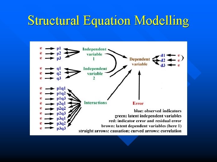
Structural Equation Modelling • • What is a "structural equation model" and how is it diagrammed? A structural equation mode is a complete path model which can be depicted in a path diagram. It differs from simple path analysis in that all variables are latent variables measured by multiple indicators which have associated error terms in addition to the residual error factor associated with the latent dependent variable. The figure below shows a structural equation model for two independents (each measured by three indicators) and their interactions (3 indicators times 3 indicators = nine interactions) as cause of one dependent (itself measured by three indicators). A SEM diagram commonly has certain standard elements: latents are ellipses, indicators are rectangles, error and residual terms are circles, single-headed arrows are causal relations (note causality goes from a latent to its indicators), and double-headed arrows are correlations between indicators or between exogenous latents. Path coefficient values may be placed on the arrows from latents to indicators, or from one latent to another, or from an error term to an indicator, or from a residual term to a latent. Each endogenous variable (the one 'Dependent variable' in the model below) has an error term, sometimes called a disturbance term or residual error, not to be confused with indicator error, e, associated with each indicator variable.

Structural Equation Modelling

Structural Equation Modelling What is a second order factor model in SEM? A second-order factor model is one with one or more latents whose indicators are themselves latents. • What is a "multi-level model"? Multi-level modelling addresses the special issue of hierarchical data (ex. , data on students and data or their classes and data on their schools). Because of the group effects involved in multi-level modelling, analysis of covariance structures requires somewhat different algorithms implemented by such software packages as HLM and ML Win. This is a variant of structural equation modelling. •

Structural Equation Modelling • • 2 SLS Two-stage least squares (2 SLS) is an estimation method which adapts OLS to handle correlated error and thus to handle non-recursive path models. LISREL, one of the leading SEM packages, uses 2 SLS to derive the starting coefficient estimates for MLE. When is a confirmatory factor analysis (CFA) model identified in SEM? CFA models in SEM have no causal paths (straight arrows in the diagram) connecting the latent variables. The latent variables may be allowed to correlate (oblique factors) or be constrained to 0 covariance (orthogonal factors). CFA analysis in SEM usually focuses on analysis of the error terms of the indicator variables. Like other models, CFA models in SEM must be identified for there to be a unique solution. In a standard CFA model each indicator is specified to load only on one factor, measurement error terms are specified to be uncorrelated with each other, and all factors are allowed to correlate with each other. One-factor standard models are identified if the factor has three or more indicators. Multifactor standard models are identified if each factor has two or more indicators.

Structural Equation Modelling • • • Non-recursive models involving all possible correlations among the disturbance terms of the endogenous variables. This introduces nonrecursivity in the form of feedback loops. Non-recursive models with variables grouped in blocks. The relation of the blocks is recursive. Variables within any block may not be recursively related, but within each block the researcher assumes the existence of all possible correlations among the disturbance terms of the endogenous variables for that block. Such a model may be identified if each block passes the tests for non-recursive models involving all possible correlations among the disturbance terms of its endogenous variables. Non-recursive models assuming only some disturbance terms of the endogenous variables are correlated.

Structural Equation Modelling What is a matrix in LISREL? In LISREL, the model is specified through inputting a set of 8 to 12 matrices of 0's and 1's which tell LISREL the structure of the model. • • • Lambda X Matrix. This specifies the paths from the latent independent variables to their observed indicators. The 1's indicate causal arrows in the model. Lambda Y Matrix. The same for the latent dependent variable(s). Theta Delta Matrix. This deals with the error terms of the independent variable indicators. For n indicators, this matrix is n-by-n, where 1's on the diagonal indicated that error variance should be estimated for that variable and 1's off the diagonal indicated correlated error (an that correlated error covariance should be estimated). Theta Epsilon Matrix. The same for the error terms of the observed dependent indicators.

Structural Equation Modelling • • • Phi Matrix. Deals with the latent independent variables, where 1's on the diagonal indicate the variance of the latent variables is to be estimated (standard practice) and 1's off the diagonal indicate correlation of the latent intependent variables (the usual situation). Gamma Matrix. The central part of the model, where 1's indicate a causal path from the latent independent variable to the latent dependent variable Beta Matrix. This matrix always has 0's on the diagonal, and 1's on the offdiagonal indicate a causal path from the column latent dependent variable to the row latent dependent variable. Psi Matrix. A 1 indicates LISREL should compute the variance of the latent residual error term, E, for the latent dependent(s). An off-diagonal 1 indicates correlated residuals among the E terms for each of the latent dependent variables. If there is only one latent dependent, then the matrix is a single "1". Kappa Matrix, KA. Used if interaction effects are modelled, a 1 means to estimate the mean of the given latent variable.

Structural Equation Modelling • • • Alpha Matrix. Used if interaction effects are modelled, a 1 means to estimate the intercept in the regression equation for the latent dependent on the latent independent variables. Tau-X Matrix. Used if interaction effects are modelled, a 1 means to estimate the intercept of the regression of the latent independent variable on its indicators. Tau-Y Matrix. Used if interaction effects are modelled, a 1 means to estimate the intercept of the regression of the latent dependent variable on its indicators.