Structural Equation Modelling Jouko Miettunen Ph D Department

Structural Equation Modelling Jouko Miettunen, Ph. D Department of Psychiatry University of Oulu e-mail: jouko. miettunen@oulu. fi 1

Topics of this presentation n Background u Factor analyses u Regression analyses n n n Theory Modeling with AMOS References 2

Structural Equation Modeling n n Based on factor analysis First studies by Karl E. Jöreskog and Dag Sörbom in 1970’s u “LISREL n n n –models” Combination of factor analysis and regression analysis Continuous and discrete predictors and outcomes Relationships among measured or latent variables 3

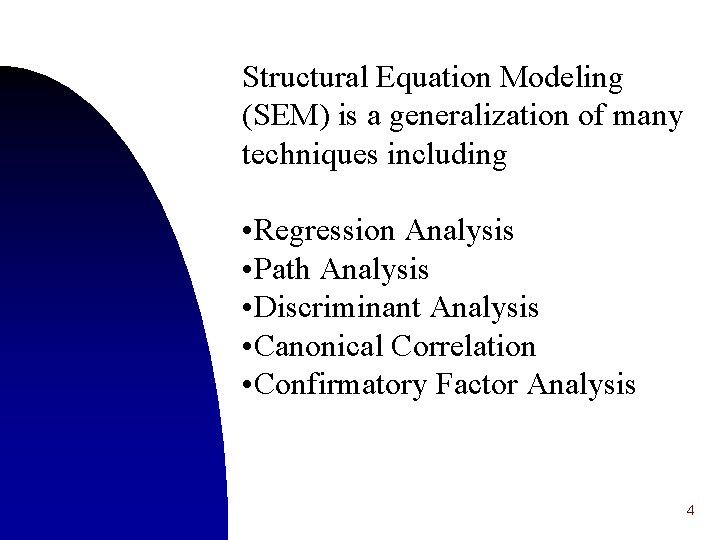
Structural Equation Modeling (SEM) is a generalization of many techniques including • Regression Analysis • Path Analysis • Discriminant Analysis • Canonical Correlation • Confirmatory Factor Analysis 4

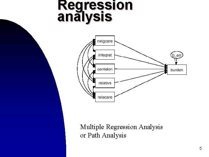
Regression analysis Multiple Regression Analysis or Path Analysis 5

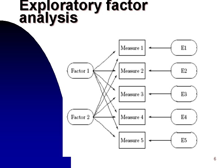
Exploratory factor analysis 6

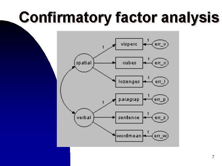
Confirmatory factor analysis 7

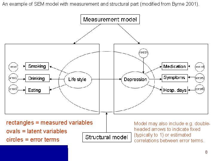
An example of SEM model with measurement and structural part (modified from Byrne 2001). rectangles = measured variables ovals = latent variables circles = error terms Model may also include e. g. doubleheaded arrows to indicate fixed (typically to 1) or estimated correlations between error terms. 8

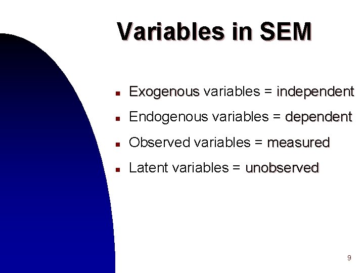
Variables in SEM n Exogenous variables = independent n Endogenous variables = dependent n Observed variables = measured n Latent variables = unobserved 9

Sample size n n n 15 cases per predictor in a standard ordinary least squares multiple regression analysis. Researchers may go as low as five cases per parameter estimate in SEM analyses, but only if the data are perfectly wellbehaved Usually 5 cases per parameter is equivalent to 15 measured variables. Bentler and Chou (1987), Stevens (1996) 10

Phases of SEM n Theoretical model u Drawing the model u Including constraints n n Model identification Estimation Fit of the model Improving model 11

Model identification n n P is # of measured variables DF = [P*(P+1)]/2 - (# of estimated parameters) If DF>0 model is over identified If DF=0 model is just identified If DF<0 model is under identified 12

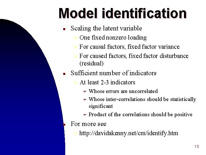
Model identification n Scaling the latent variable One fixed nonzero loading u For causal factors, fixed factor variance u For caused factors, fixed factor disturbance (residual) u n Sufficient number of indicators u At least 2 -3 indicators Whose errors are uncorrelated F Whose inter-correlations should be statistically significant F Product of the correlations should be positive F n For more see u http: //davidakenny. net/cm/identify. htm 13

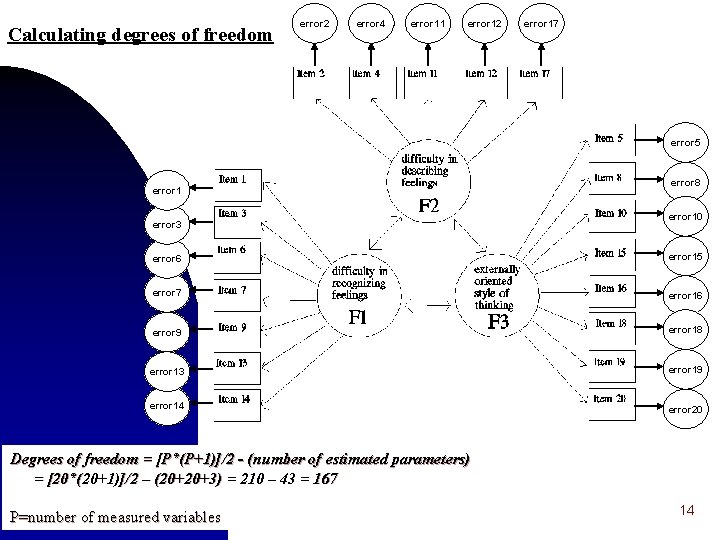
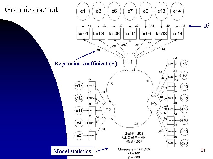
Calculating degrees of freedom error 2 error 4 error 11 error 12 error 17 error 5 error 1 error 3 error 8 error 10 error 6 error 15 error 7 error 16 error 9 error 18 error 13 error 19 error 14 error 20 Degrees of freedom = [P*(P+1)]/2 - (number of estimated parameters) = [20*(20+1)]/2 – (20+20+3) = 210 – 43 = 167 P=number of measured variables 14

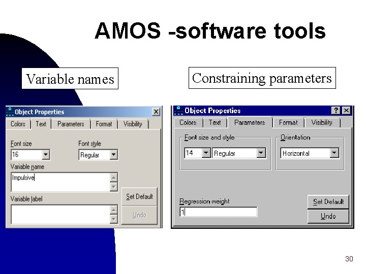
Constraining parameters § Typically some of the factor loadings are constrained or fixed to be zero. § For each factor it is also necessary to fix one loading to the value one in order to give the latent factor an interpretable scale. § One solution is to fix the variance of all factors to one and then estimate all factor loadings. 15

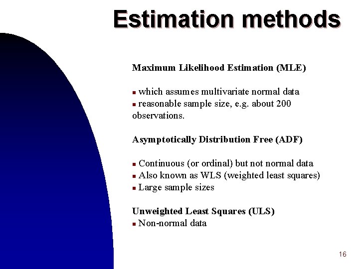
Estimation methods Maximum Likelihood Estimation (MLE) which assumes multivariate normal data n reasonable sample size, e. g. about 200 observations. n Asymptotically Distribution Free (ADF) Continuous (or ordinal) but normal data n Also known as WLS (weighted least squares) n Large sample sizes n Unweighted Least Squares (ULS) n Non-normal data 16

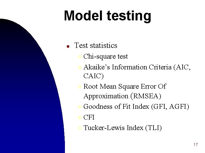
Model testing n Test statistics u Chi-square test u Akaike’s Information Criteria (AIC, CAIC) u Root Mean Square Error Of Approximation (RMSEA) u Goodness of Fit Index (GFI, AGFI) u CFI u Tucker-Lewis Index (TLI) 17

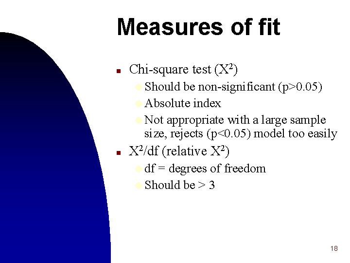
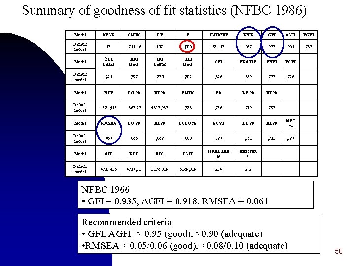
Measures of fit n Chi-square test (X 2) u Should be non-significant (p>0. 05) u Absolute index u Not appropriate with a large sample size, rejects (p<0. 05) model too easily n X 2/df (relative X 2) u df = degrees of freedom u Should be > 3 18

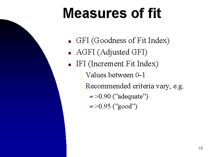
Measures of fit n n n GFI (Goodness of Fit Index) AGFI (Adjusted GFI) IFI (Increment Fit Index) u Values between 0 -1 u Recommended criteria vary, e. g. F >0. 90 (”adequate”) F >0. 95 (”good”) 19

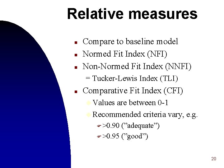
Relative measures n n n Compare to baseline model Normed Fit Index (NFI) Non-Normed Fit Index (NNFI) = Tucker-Lewis Index (TLI) n Comparative Fit Index (CFI) u Values are between 0 -1 u Recommended criteria vary, e. g. F >0. 90 (”adequate”) F >0. 95 (”good”) 20

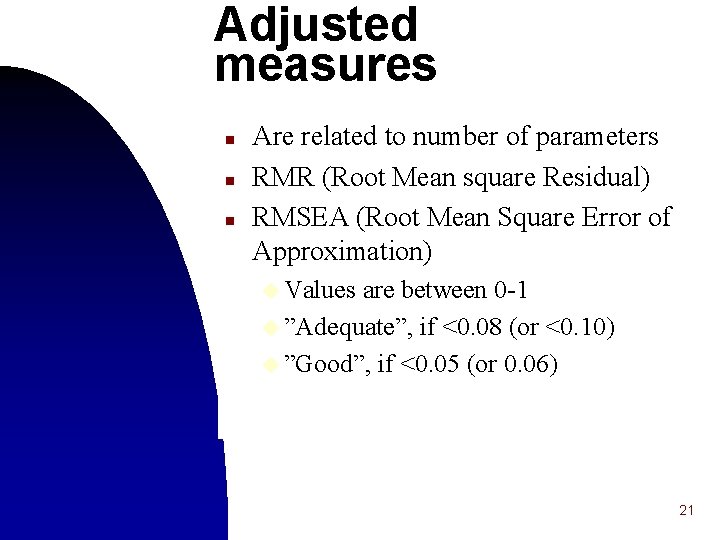
Adjusted measures n n n Are related to number of parameters RMR (Root Mean square Residual) RMSEA (Root Mean Square Error of Approximation) u Values are between 0 -1 u ”Adequate”, if <0. 08 (or <0. 10) u ”Good”, if <0. 05 (or 0. 06) 21

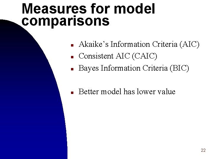
Measures for model comparisons n Akaike’s Information Criteria (AIC) Consistent AIC (CAIC) Bayes Information Criteria (BIC) n Better model has lower value n n 22

Modification indices § If the fit of a model is not adequate, you can delete non-significant parameters and add other parameters that will improve the fit. § The value given is the minimum amount that the chi-square statistic is expected to decrease if the corresponding parameter is freed. § Theoretical justification is needed. 23

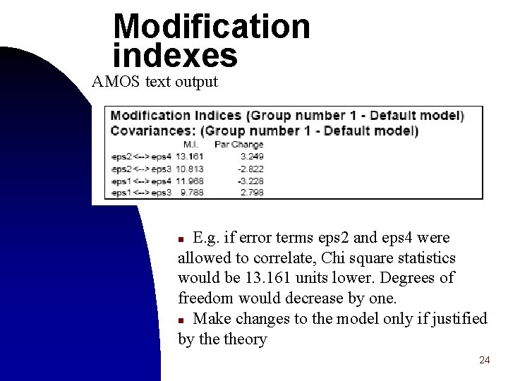
Modification indexes AMOS text output E. g. if error terms eps 2 and eps 4 were allowed to correlate, Chi square statistics would be 13. 161 units lower. Degrees of freedom would decrease by one. n Make changes to the model only if justified by theory n 24

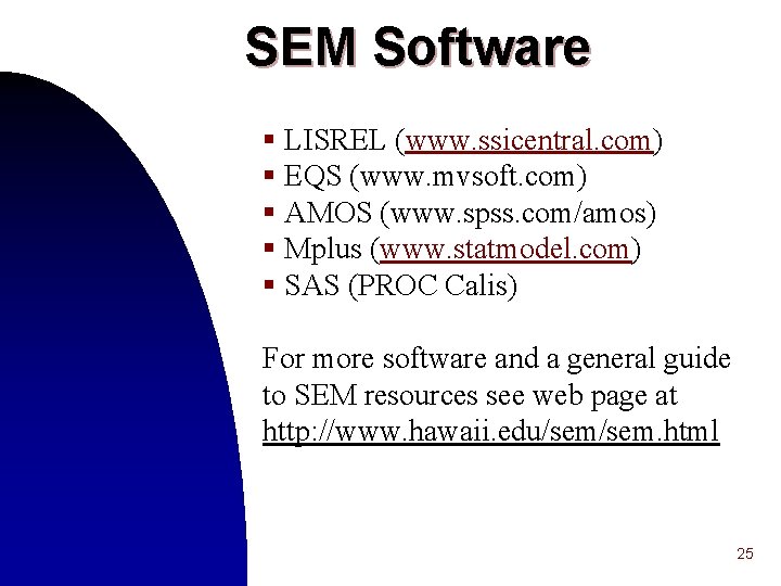
SEM Software § LISREL (www. ssicentral. com) § EQS (www. mvsoft. com) § AMOS (www. spss. com/amos) § Mplus (www. statmodel. com) § SAS (PROC Calis) For more software and a general guide to SEM resources see web page at http: //www. hawaii. edu/sem. html 25

SEM analyses in AMOS Graphics u u n draw SEM graphs runs SEM models using graphs AMOS Program Editor u runs SEM models using syntax 26

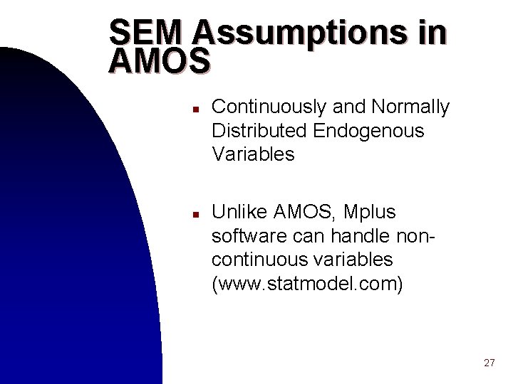
SEM Assumptions in AMOS n n Continuously and Normally Distributed Endogenous Variables Unlike AMOS, Mplus software can handle noncontinuous variables (www. statmodel. com) 27

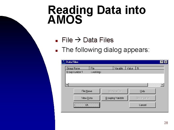
Reading Data into AMOS n n File Data Files The following dialog appears: 28

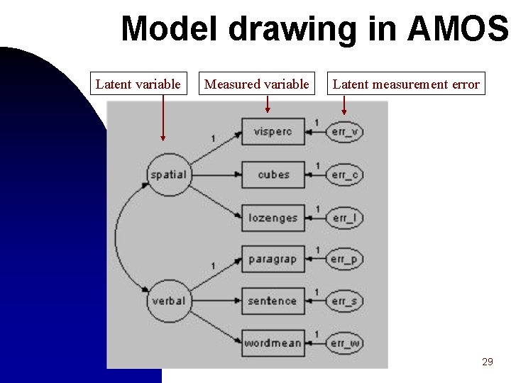
Model drawing in AMOS Latent variable Measured variable Latent measurement error 29

AMOS -software tools Variable names Constraining parameters 30

Icons in AMOS 31

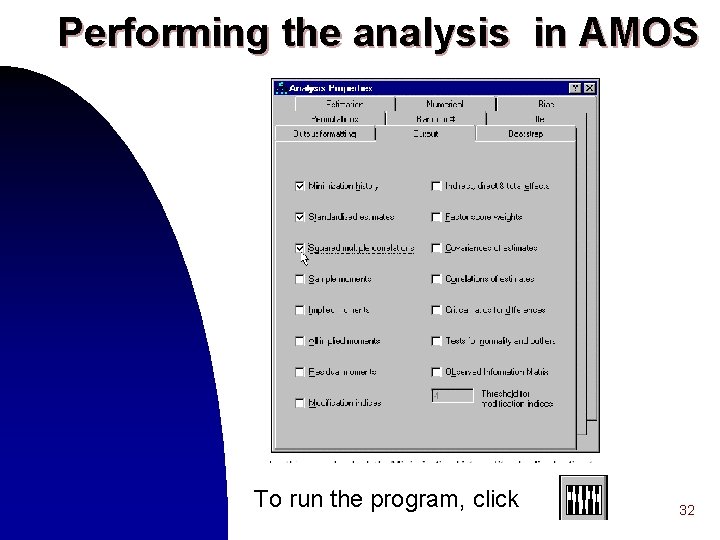
Performing the analysis in AMOS To run the program, click 32

Presentation of model results in AMOS n Text output n Graphics output n Examples later 33

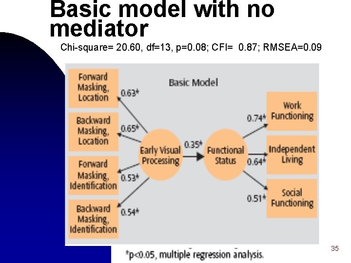
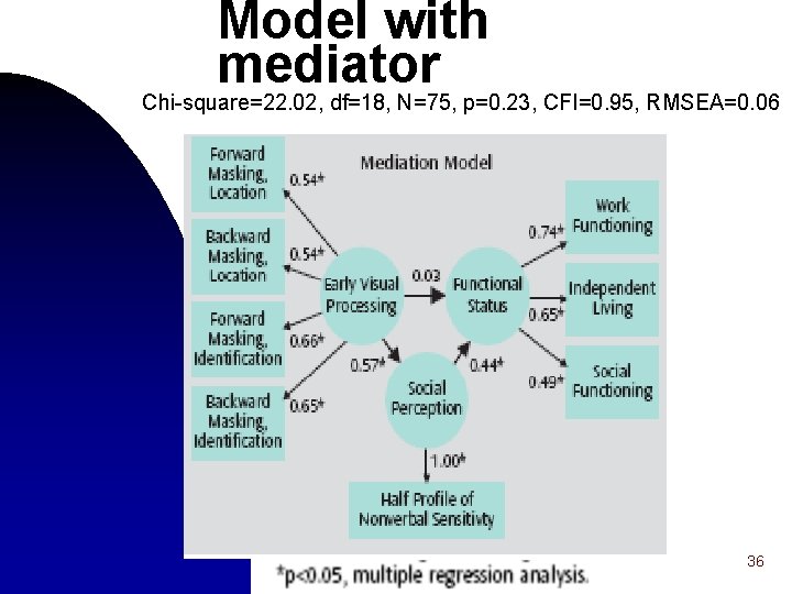
Example I Social Perception as a Mediator of the Influence of Early Visual Processing on Functional Status in Schizophrenia The authors used SEM to test whether one aspect of social cognition (social perception) mediates relations between visual perception and functional status in patients with schizophrenia (N=75). SEM supported social perception as a mediator of relations between early visual processing and functional status in schizophrenia. Direct relationship between early visual processing and functional status was significant in a model that did not include social perception but was not significant in the mediation model that included social perception. Sergi et al. Am J Psychiatry 2006: 163: 448 -54 34

Basic model with no mediator Chi-square= 20. 60, df=13, p=0. 08; CFI= 0. 87; RMSEA=0. 09 35

Model with mediator Chi-square=22. 02, df=18, N=75, p=0. 23, CFI=0. 95, RMSEA=0. 06 36

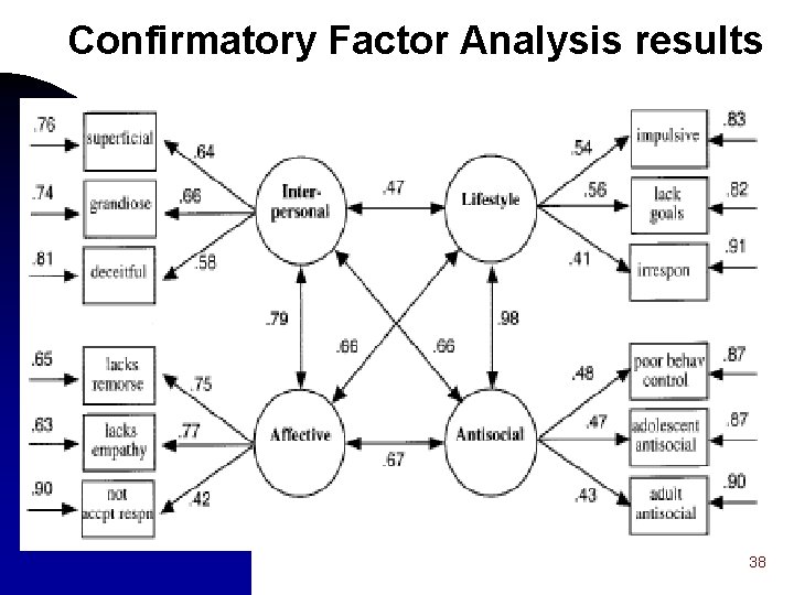
Example II Confirmatory Factor Analysis of the Psychopathy Checklist: Screening Version in Offenders With Axis I Disorders One hundred forty-nine inpatients within a maximum security psychiatric facility were assessed with the Psychopathy Checklist: Screening Version. Within the total sample, 68% had a psychotic disorder and 30% met criteria for psychopathy. Using CFA, the authors tested the 2 -, 3 - and 4 -factor models. Results indicated good fit for each model, with the 4 factor model showing best overall fit. SEM was used to determine which psychopathy factors predicted 6 month follow-up of inpatient aggression. The 2 -, 3 -, and 4 -factor models, respectively, accounted for 16%, 27%, and 31% of the variance in aggression. Hill et al. Psychol Assessm 2004: 16: 90 -5. 37

Confirmatory Factor Analysis results 38

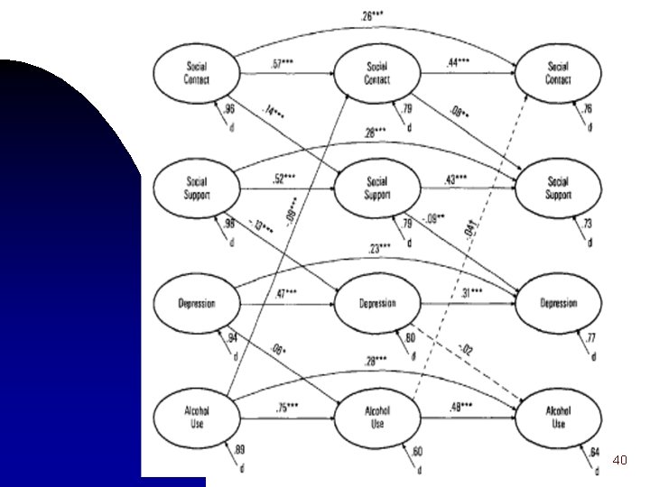
Example III A Longitudinal Model of Social Contact, Social Support, Depression, and Alcohol Use The longitudinal relations among social contact, perceived social support, depression, and alcohol use were examined. A random sample of 1, 192 adults. Results revealed that (a) social contact was positively related to perceived social support; (b) perceived social support was negatively related to depression; and (c) depression was positively related to alcohol use for 1 of 2 longitudinal lags. There was partial support for the feedback hypothesis that increased alcohol use leads to decreased contact with family and friends. Peirce et al. Health Psychol 2000: 19: 28 -38. 39

40

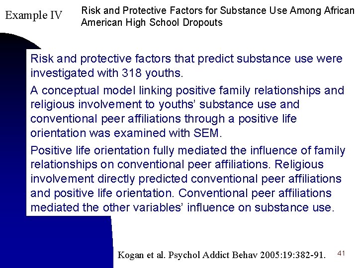
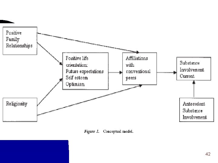
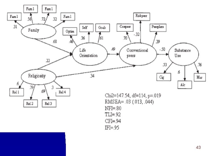
Example IV Risk and Protective Factors for Substance Use Among African American High School Dropouts Risk and protective factors that predict substance use were investigated with 318 youths. A conceptual model linking positive family relationships and religious involvement to youths’ substance use and conventional peer affiliations through a positive life orientation was examined with SEM. Positive life orientation fully mediated the influence of family relationships on conventional peer affiliations. Religious involvement directly predicted conventional peer affiliations and positive life orientation. Conventional peer affiliations mediated the other variables’ influence on substance use. Kogan et al. Psychol Addict Behav 2005: 19: 382 -91. 41

42

43

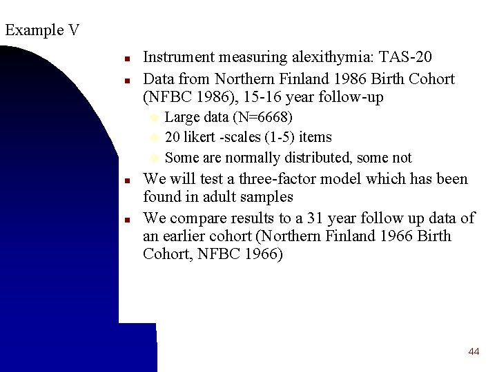
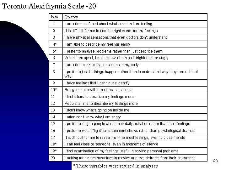
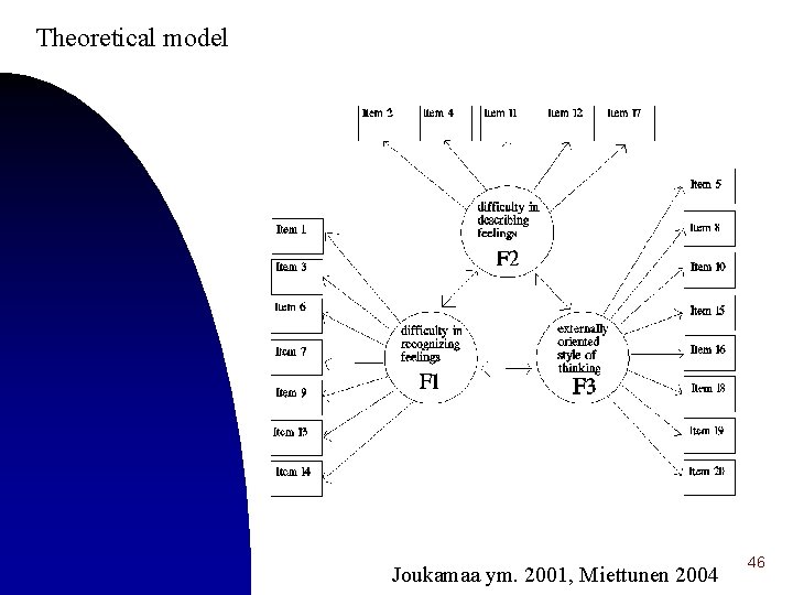
Example V n n Instrument measuring alexithymia: TAS-20 Data from Northern Finland 1986 Birth Cohort (NFBC 1986), 15 -16 year follow-up Large data (N=6668) u 20 likert -scales (1 -5) items u Some are normally distributed, some not u n n We will test a three-factor model which has been found in adult samples We compare results to a 31 year follow up data of an earlier cohort (Northern Finland 1966 Birth Cohort, NFBC 1966) 44

Toronto Alexithymia Scale -20 Item Question 1 I am often confused about what emotion I am feeling 2 It is difficult for me to find the right words for my feelings 3 I have physical sensations that even doctors don’t understand 4* I am able to describe my feelings easily 5* I prefer to analyze problems rather than just describe them 6 When I am upset, I don’t know if I am sad, frightened, or angry 7 I am often puzzled by sensations in my body 8 I prefer to just let things happen rather than to understand why they turn out that way 9 I have feelings that I can’t quite identify 10* Being in touch with emotions is essential 11 I find it hard to describe my feelings more 12 People tell me to describe my feelings more 13 I don’t know what’s going on inside me 14 I often don’t know why I am angry 15 I prefer talking to people about their daily activities rather than their feelings 16 I prefer to watch “light” entertainment shows rather than psychological dramas 17 It is difficult for me to reveal my innermost feelings, even to close friends 18* I can feel close to someone, even in moments of silence 19* I find examination of my feelings useful in solving personal problems 20 Looking for hidden meanings in movies or plays distracts from their enjoyment * These variables were revised in analyses 45

Theoretical model Joukamaa ym. 2001, Miettunen 2004 46

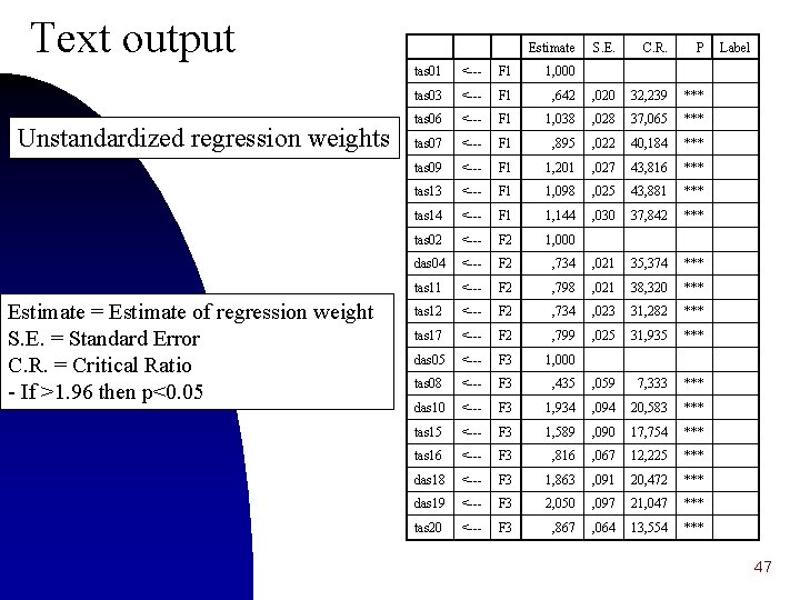
Text output Unstandardized regression weights Estimate = Estimate of regression weight S. E. = Standard Error C. R. = Critical Ratio - If >1. 96 then p<0. 05 Estimate S. E. C. R. P tas 01 <--- F 1 1, 000 tas 03 <--- F 1 , 642 , 020 32, 239 *** tas 06 <--- F 1 1, 038 , 028 37, 065 *** tas 07 <--- F 1 , 895 , 022 40, 184 *** tas 09 <--- F 1 1, 201 , 027 43, 816 *** tas 13 <--- F 1 1, 098 , 025 43, 881 *** tas 14 <--- F 1 1, 144 , 030 37, 842 *** tas 02 <--- F 2 1, 000 das 04 <--- F 2 , 734 , 021 35, 374 *** tas 11 <--- F 2 , 798 , 021 38, 320 *** tas 12 <--- F 2 , 734 , 023 31, 282 *** tas 17 <--- F 2 , 799 , 025 31, 935 *** das 05 <--- F 3 1, 000 tas 08 <--- F 3 , 435 , 059 7, 333 *** das 10 <--- F 3 1, 934 , 094 20, 583 *** tas 15 <--- F 3 1, 589 , 090 17, 754 *** tas 16 <--- F 3 , 816 , 067 12, 225 *** das 18 <--- F 3 1, 863 , 091 20, 472 *** das 19 <--- F 3 2, 050 , 097 21, 047 *** tas 20 <--- F 3 , 867 , 064 13, 554 *** Label 47

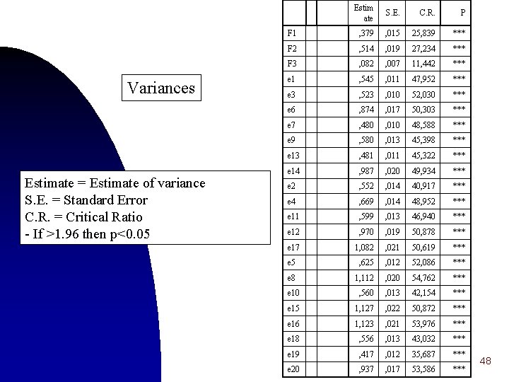
Variances Estimate = Estimate of variance S. E. = Standard Error C. R. = Critical Ratio - If >1. 96 then p<0. 05 Estim ate S. E. C. R. P F 1 , 379 , 015 25, 839 *** F 2 , 514 , 019 27, 234 *** F 3 , 082 , 007 11, 442 *** e 1 , 545 , 011 47, 952 *** e 3 , 523 , 010 52, 030 *** e 6 , 874 , 017 50, 303 *** e 7 , 480 , 010 48, 588 *** e 9 , 580 , 013 45, 398 *** e 13 , 481 , 011 45, 322 *** e 14 , 987 , 020 49, 934 *** e 2 , 552 , 014 40, 917 *** e 4 , 669 , 014 48, 952 *** e 11 , 599 , 013 46, 940 *** e 12 , 970 , 019 50, 878 *** e 17 1, 082 , 021 50, 619 *** e 5 , 625 , 012 52, 086 *** e 8 1, 112 , 020 54, 762 *** e 10 , 560 , 013 42, 154 *** e 15 1, 127 , 022 50, 872 *** e 16 1, 123 , 021 53, 976 *** e 18 , 556 , 013 43, 032 *** e 19 , 417 , 012 35, 687 *** e 20 , 937 , 017 53, 586 *** 48

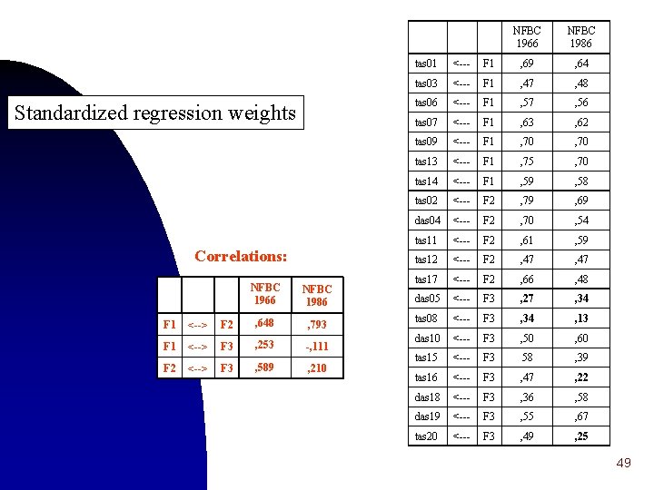
Standardized regression weights Correlations: NFBC 1966 NFBC 1986 F 1 <--> F 2 , 648 , 793 F 1 <--> F 3 , 253 -, 111 F 2 <--> F 3 , 589 , 210 NFBC 1966 NFBC 1986 tas 01 <--- F 1 , 69 , 64 tas 03 <--- F 1 , 47 , 48 tas 06 <--- F 1 , 57 , 56 tas 07 <--- F 1 , 63 , 62 tas 09 <--- F 1 , 70 tas 13 <--- F 1 , 75 , 70 tas 14 <--- F 1 , 59 , 58 tas 02 <--- F 2 , 79 , 69 das 04 <--- F 2 , 70 , 54 tas 11 <--- F 2 , 61 , 59 tas 12 <--- F 2 , 47 tas 17 <--- F 2 , 66 , 48 das 05 <--- F 3 , 27 , 34 tas 08 <--- F 3 , 34 , 13 das 10 <--- F 3 , 50 , 60 tas 15 <--- F 3 58 , 39 tas 16 <--- F 3 , 47 , 22 das 18 <--- F 3 , 36 , 58 das 19 <--- F 3 , 55 , 67 tas 20 <--- F 3 , 49 , 25 49

Summary of goodness of fit statistics (NFBC 1986) Model NPAR CMIN DF P CMIN/DF RMR GFI AGFI PGFI Default model 43 4751, 46 167 , 000 28, 452 , 067 , 922 , 901 , 733 Model NFI Delta 1 RFI rho 1 IFI Delta 2 TLI rho 2 CFI PRATIO PNFI PCFI Default model , 821 , 797 , 826 , 802 , 826 , 879 , 722 , 726 Model NCP LO 90 HI 90 FMIN F 0 LO 90 HI 90 Default model 4584, 455 4363, 23 4812, 932 , 783 , 756 , 719 , 793 Model RMSEA LO 90 HI 90 PCLOSE ECVI LO 90 HI 90 MEC VI Default model , 067 , 066 , 069 , 000 , 797 , 761 , 835 , 797 Model AIC BCC BIC CAIC HOELTER. 05 HOELTER. 01 Default model 4837, 455 4837, 75 5126, 019 5169, 019 254 272 NFBC 1966 • GFI = 0. 935, AGFI = 0. 918, RMSEA = 0. 061 Recommended criteria • GFI, AGFI > 0. 95 (good), >0. 90 (adequate) • RMSEA < 0. 05/0. 06 (good), <0. 08/0. 10 (adequate) 50

Graphics output R 2 Regression coefficient (R) Model statistics 51

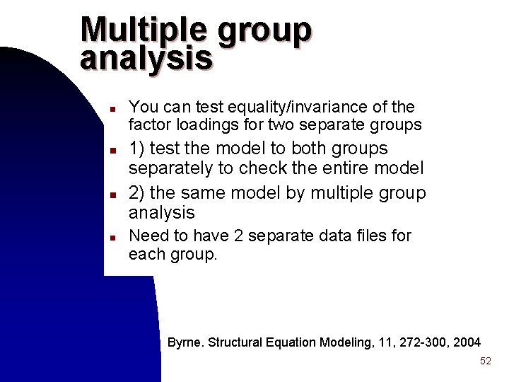
Multiple group analysis n n You can test equality/invariance of the factor loadings for two separate groups 1) test the model to both groups separately to check the entire model 2) the same model by multiple group analysis Need to have 2 separate data files for each group. Byrne. Structural Equation Modeling, 11, 272 -300, 2004 52

Handling Missing data in SEM n n Listwise or pairwise Mean substitution Regression methods Expectation Maximization (EM) approach Best methods n Full Information Maximum Likelihood (FIML) n Multiple imputation (MI) 53

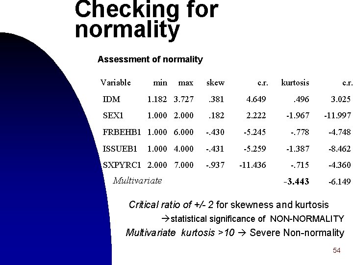
Checking for normality Assessment of normality Variable min max skew c. r. kurtosis c. r. IDM 1. 182 3. 727 . 381 4. 649 . 496 3. 025 SEX 1 1. 000 2. 000 . 182 2. 222 -1. 967 -11. 997 FRBEHB 1 1. 000 6. 000 -. 430 -5. 245 -. 778 -4. 748 ISSUEB 1 1. 000 4. 000 -. 431 -5. 259 -1. 387 -8. 462 SXPYRC 1 2. 000 7. 000 -. 937 -11. 436 -. 715 -4. 360 -3. 443 -6. 149 Multivariate Critical ratio of +/- 2 for skewness and kurtosis statistical significance of NON-NORMALITY Multivariate kurtosis >10 Severe Non-normality 54

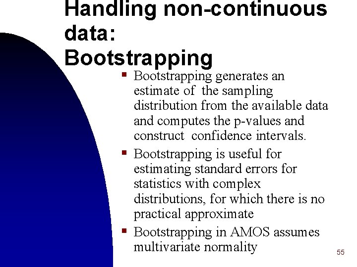
Handling non-continuous data: Bootstrapping § Bootstrapping generates an estimate of the sampling distribution from the available data and computes the p-values and construct confidence intervals. § Bootstrapping is useful for estimating standard errors for statistics with complex distributions, for which there is no practical approximate § Bootstrapping in AMOS assumes multivariate normality 55

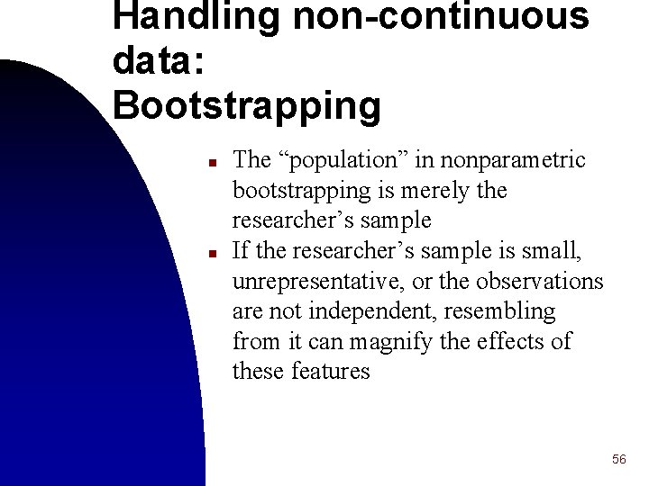
Handling non-continuous data: Bootstrapping n n The “population” in nonparametric bootstrapping is merely the researcher’s sample If the researcher’s sample is small, unrepresentative, or the observations are not independent, resembling from it can magnify the effects of these features 56

Problems in interpreting SEM § Statistical assumptions and required sample sizes are needed to have confidence in the results § Misrepresentation of causal relationships. Most applications of SEM are on non-experimental data but many nevertheless interpret the final model as causal. 57

Referenc es n n Barrett. Structural Equation Modelling: Adjudging model fit. Pers Indiv Diff, In press. Bentler & Chou. Practical issues in structural modeling. Sociological Methods and Research 16(1): 78 -117, 1987. Bentler & Stein. Structural equation models in medical research. Stat Methods Med Res 1: 159– 181, 1992. Bollen. Structural equations with latent variables. John Wiley & Sons, Inc, New York, 1989. 58

References n n Byrne. Structural Equation Modeling with AMOS: Basic Concepts, Applications, and Programming. Lawrence Erlbaum Associates, Inc. , 2001 Finch & West. The investigation of personality structure: statistical models. J Res Pers 31: 439– 485, 1997. Mac. Callum & Austin. Applications of structural equation modeling in psychological research. Annu Rev Psychol 51: 201– 226, 2000. De Stavola et al. Statistical issues in life course epidemiology. Am J Epidemiol 163: 84 -96, 2006. 59

References n n n Stevens. Applied multivariate statistics for the social sciences. Mahwah, NJ: Lawrence Erlbaum Publishers, 1996. Wolfle. The introduction of path analysis to the social sciences, and some emergent themes: an annotated bibliography. Struct Equation Model 10(1): 1 -34, 2003. More references etc. in internet. u u u www. statmodel. com www. spss. com/amos http: //www. upa. pdx. edu/IOA/newsom/semrefs. ht m http: //amosdevelopment. com/Amos. Citations. htm http: //www 2. chass. ncsu. edu/garson/pa 765/structur. htm 60