Statistics and Calculus 1 Statistics in Maxima and

Statistics and Calculus 1

Statistics in Maxima and Excel 2

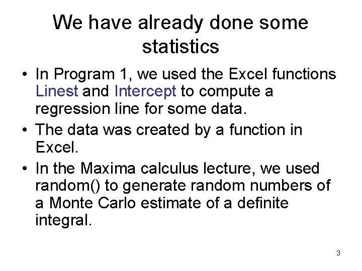
We have already done some statistics • In Program 1, we used the Excel functions Linest and Intercept to compute a regression line for some data. • The data was created by a function in Excel. • In the Maxima calculus lecture, we used random() to generate random numbers of a Monte Carlo estimate of a definite integral. 3

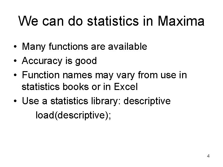
We can do statistics in Maxima • Many functions are available • Accuracy is good • Function names may vary from use in statistics books or in Excel • Use a statistics library: descriptive load(descriptive); 4

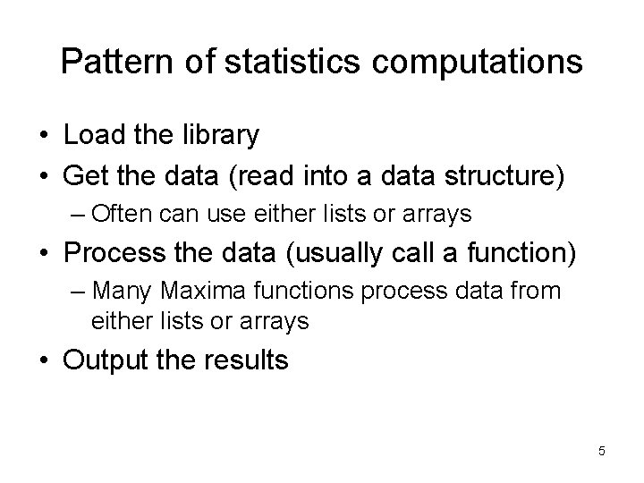
Pattern of statistics computations • Load the library • Get the data (read into a data structure) – Often can use either lists or arrays • Process the data (usually call a function) – Many Maxima functions process data from either lists or arrays • Output the results 5

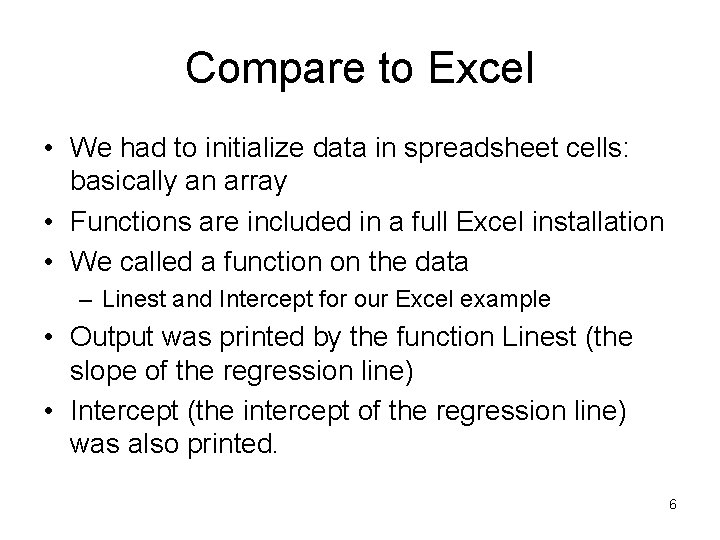
Compare to Excel • We had to initialize data in spreadsheet cells: basically an array • Functions are included in a full Excel installation • We called a function on the data – Linest and Intercept for our Excel example • Output was printed by the function Linest (the slope of the regression line) • Intercept (the intercept of the regression line) was also printed. 6

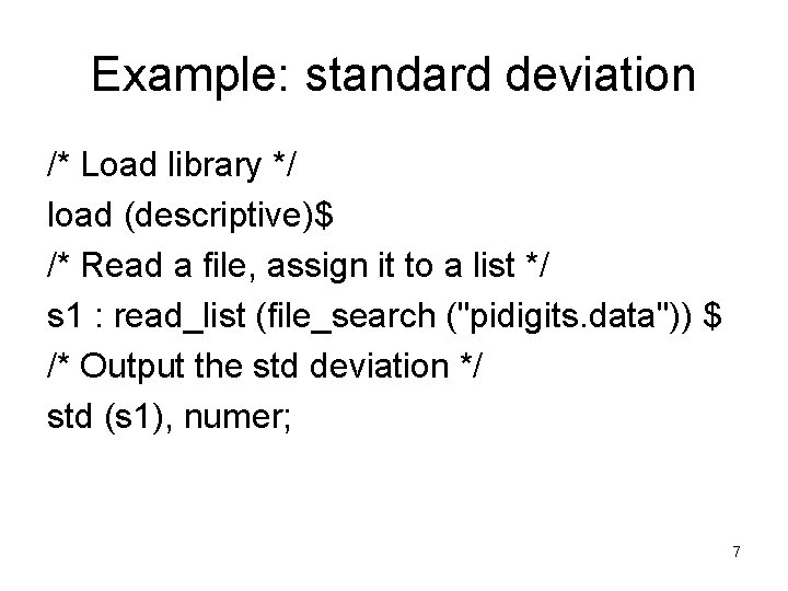
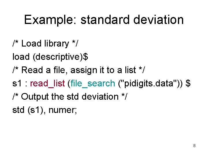
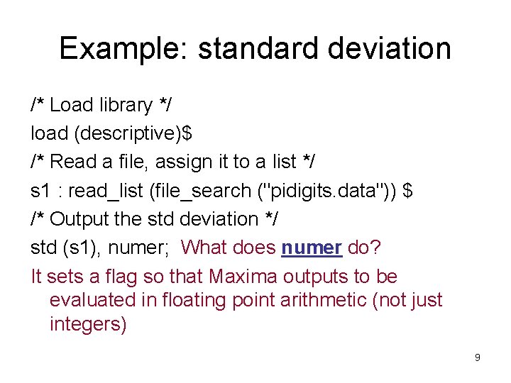
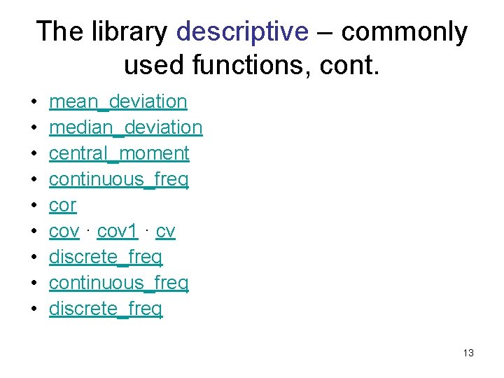
Example: standard deviation /* Load library */ load (descriptive)$ /* Read a file, assign it to a list */ s 1 : read_list (file_search ("pidigits. data")) $ /* Output the std deviation */ std (s 1), numer; 7

Example: standard deviation /* Load library */ load (descriptive)$ /* Read a file, assign it to a list */ s 1 : read_list (file_search ("pidigits. data")) $ /* Output the std deviation */ std (s 1), numer; 8

Example: standard deviation /* Load library */ load (descriptive)$ /* Read a file, assign it to a list */ s 1 : read_list (file_search ("pidigits. data")) $ /* Output the std deviation */ std (s 1), numer; What does numer do? It sets a flag so that Maxima outputs to be evaluated in floating point arithmetic (not just integers) 9

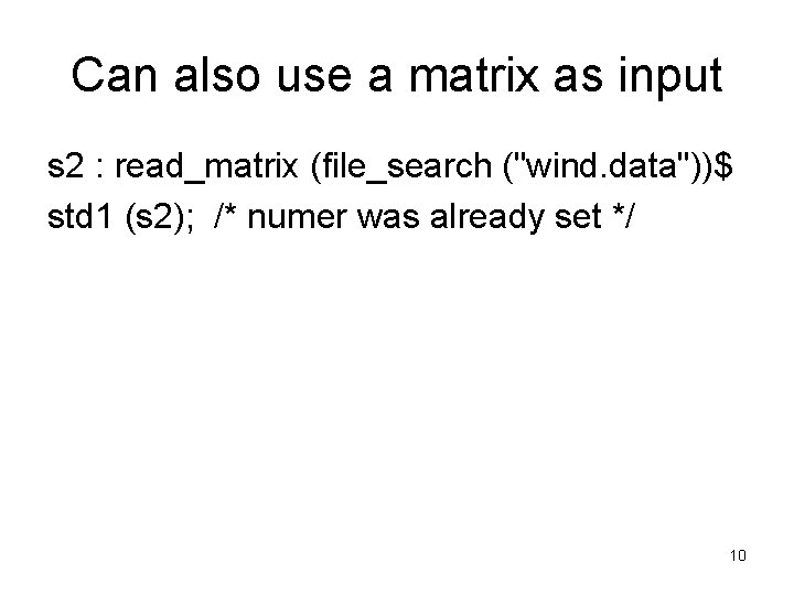
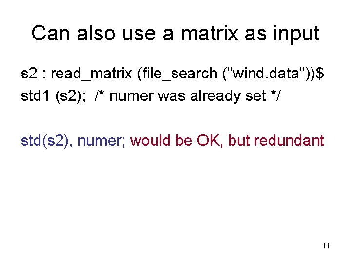
Can also use a matrix as input s 2 : read_matrix (file_search ("wind. data"))$ std 1 (s 2); /* numer was already set */ 10

Can also use a matrix as input s 2 : read_matrix (file_search ("wind. data"))$ std 1 (s 2); /* numer was already set */ std(s 2), numer; would be OK, but redundant 11

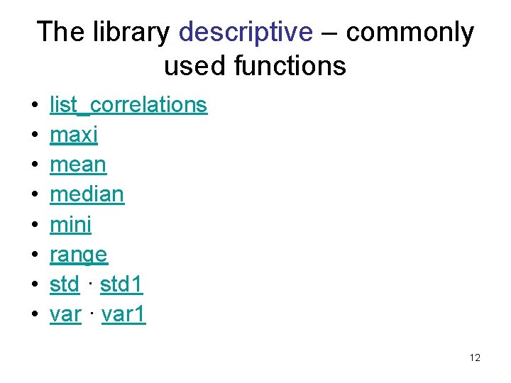
The library descriptive – commonly used functions • • list_correlations maxi mean median mini range std · std 1 var · var 1 12

The library descriptive – commonly used functions, cont. • • • mean_deviation median_deviation central_moment continuous_freq cor cov · cov 1 · cv discrete_freq continuous_freq discrete_freq 13

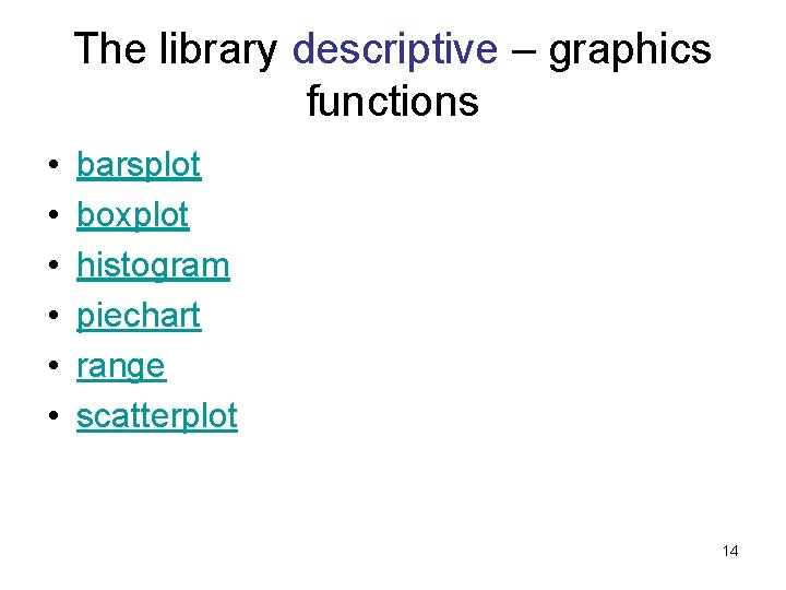
The library descriptive – graphics functions • • • barsplot boxplot histogram piechart range scatterplot 14

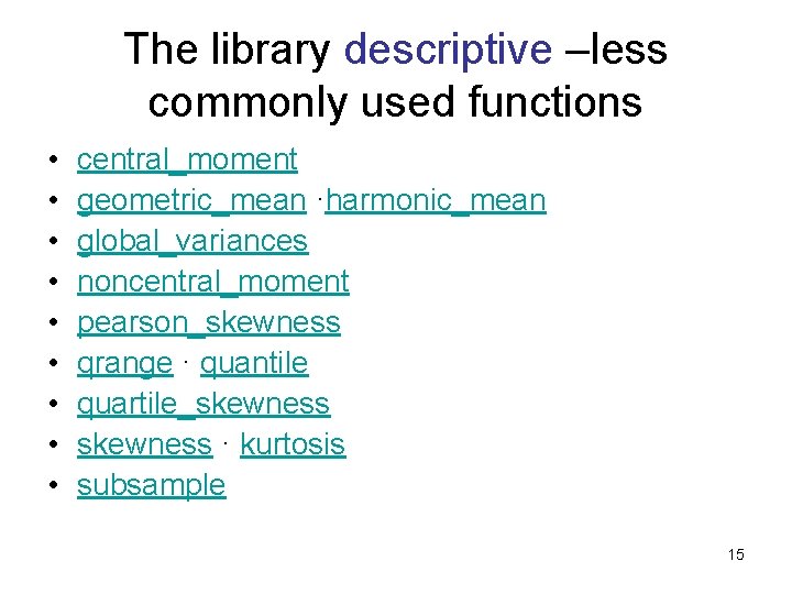
The library descriptive –less commonly used functions • • • central_moment geometric_mean ·harmonic_mean global_variances noncentral_moment pearson_skewness qrange · quantile quartile_skewness · kurtosis subsample 15

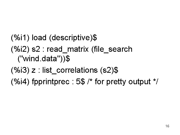
(%i 1) load (descriptive)$ (%i 2) s 2 : read_matrix (file_search ("wind. data"))$ (%i 3) z : list_correlations (s 2)$ (%i 4) fpprintprec : 5$ /* for pretty output */ 16

(%i 5) z[1]; /* precision matrix */ [. 38486 -. 13856 -. 15626 -. 10239. 031179 ] [ -. 13856. 34107 -. 15233. 038447 -. 052842 ] [ ] 17

Output [ -. 15626 -. 15233. 47296 -. 024816 -. 10054 ] [ -. 10239. 038447 -. 024816. 10937 -. 034033 ] [. 031179 -. 052842 -. 10054 -. 034033. 14834 ] 18

This is related to our Excel example • Requires normalization of Excel example to have mean =0, std dev = 1 • This forces our Linest slope to be normalized to be between 0 and 1. 19

Conclusion • There are many statistical packages in Maxima 20

How are data usually obtained? 1. By using a closed-form expression, such as sin(x) * sqrt(1 + x ^3)/x 2. By using data sets provided by other scientists or researchers 3. By continuous data acquisition, such as lab experiments 4. By using data produced by other applications (Excel to Maxima, Maxima to Excel, …) 21

Using data files • • Being able to read data from files is critical Being able to write data to files is critical File formats must be standard Most common standards: – space-delimited – tab-delimited – comma-delimited 22

Conclusion 2 • Engineers and scientists need to be able to use several different techniques to solve problems, depending on the context and the tools available. 23

Calculus in Maxima 24

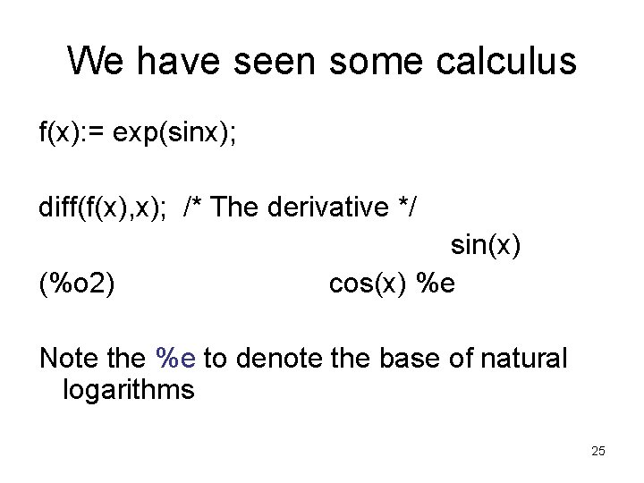
We have seen some calculus f(x): = exp(sinx); diff(f(x), x); /* The derivative */ (%o 2) sin(x) cos(x) %e Note the %e to denote the base of natural logarithms 25

Critical Points 26

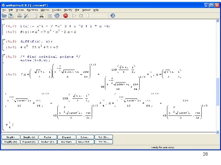
• Determine where the derivative of a function has the value 0. • We did this with graphs of a function made using gnuplot by tracking the cursor position 27

28

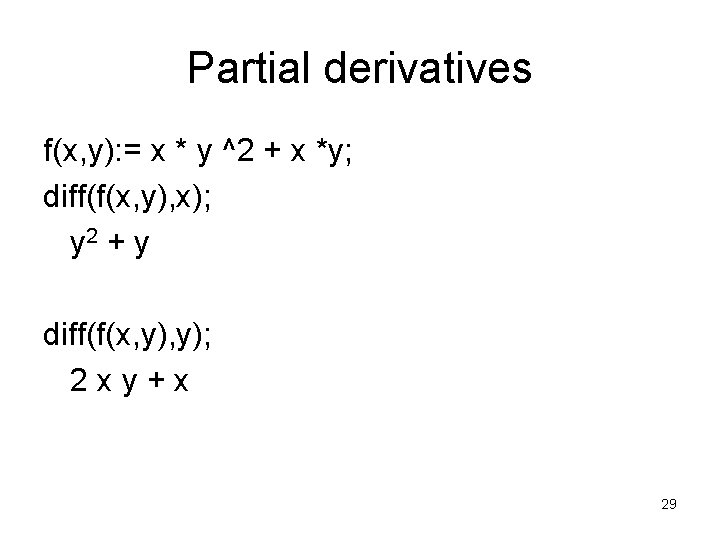
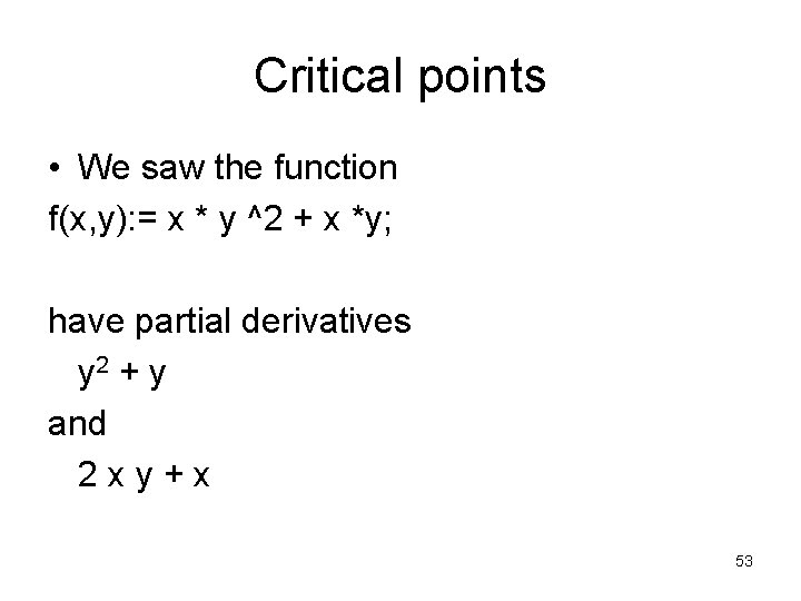
Partial derivatives f(x, y): = x * y ^2 + x *y; diff(f(x, y), x); y 2 + y diff(f(x, y); 2 xy+x 29

Integral Calculus 30

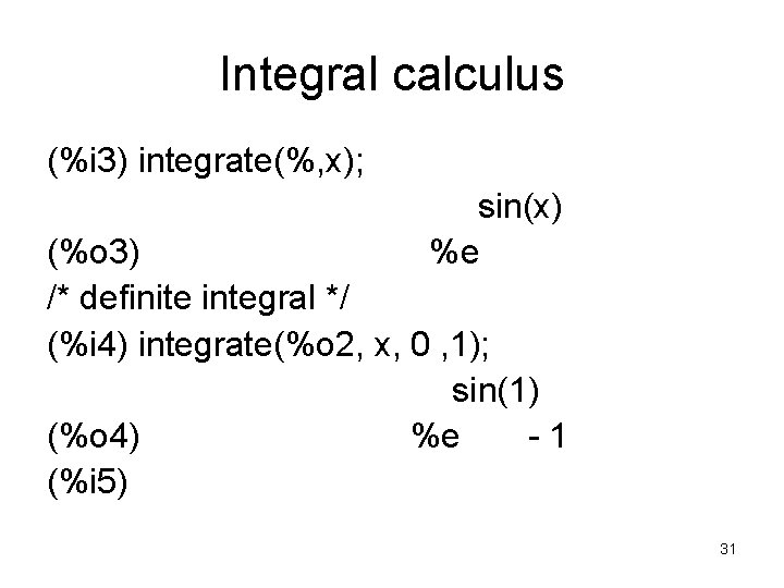
Integral calculus (%i 3) integrate(%, x); sin(x) %e (%o 3) /* definite integral */ (%i 4) integrate(%o 2, x, 0 , 1); sin(1) (%o 4) %e -1 (%i 5) 31

Maxima calculates better than you! • In the 1960 s – early 1990 s, most calculus books had 10+ pages devoted to tables of integrals, often much more. • Many problems were painstaking, requiring many steps. 32

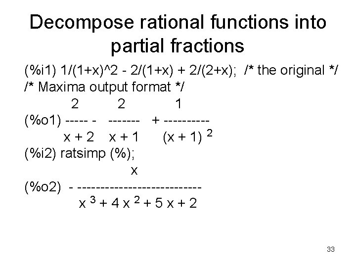
Decompose rational functions into partial fractions (%i 1) 1/(1+x)^2 - 2/(1+x) + 2/(2+x); /* the original */ /* Maxima output format */ 2 2 1 (%o 1) ----- - ------- + -----x+2 x+1 (x + 1) 2 (%i 2) ratsimp (%); x (%o 2) - -------------x 3+4 x 2+5 x+2 33

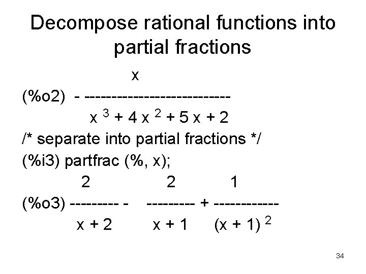
Decompose rational functions into partial fractions x (%o 2) - -------------x 3+4 x 2+5 x+2 /* separate into partial fractions */ (%i 3) partfrac (%, x); 2 2 1 (%o 3) ----- - ----- + ------x+2 x+1 (x + 1) 2 34

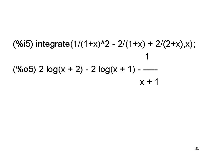
(%i 5) integrate(1/(1+x)^2 - 2/(1+x) + 2/(2+x), x); 1 (%o 5) 2 log(x + 2) - 2 log(x + 1) - ----x+1 35

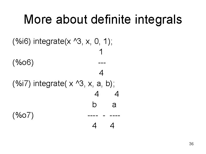
More about definite integrals (%i 6) integrate(x ^3, x, 0, 1); 1 (%o 6) --4 (%i 7) integrate( x ^3, x, a, b); 4 4 b a (%o 7) ---- - ---4 4 36

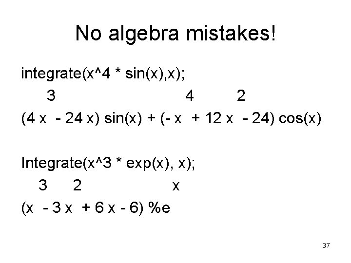
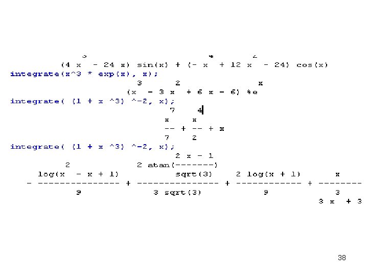
No algebra mistakes! integrate(x^4 * sin(x), x); 3 4 2 (4 x - 24 x) sin(x) + (- x + 12 x - 24) cos(x) Integrate(x^3 * exp(x), x); 3 2 x (x - 3 x + 6 x - 6) %e 37

38

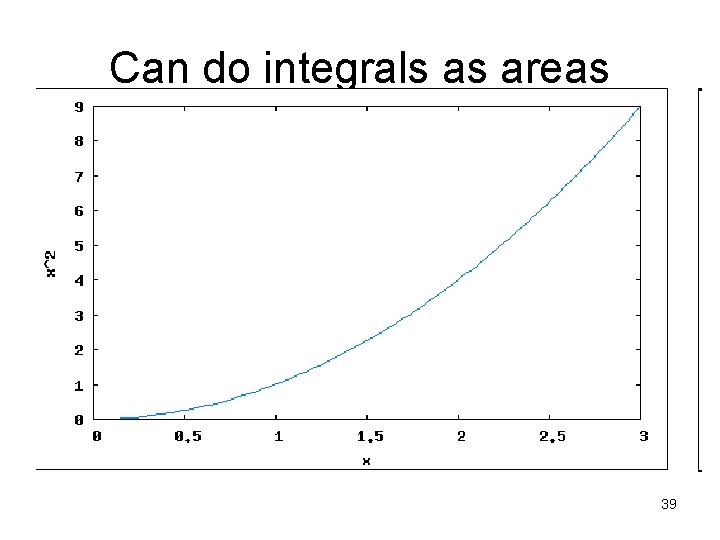
Can do integrals as areas 39

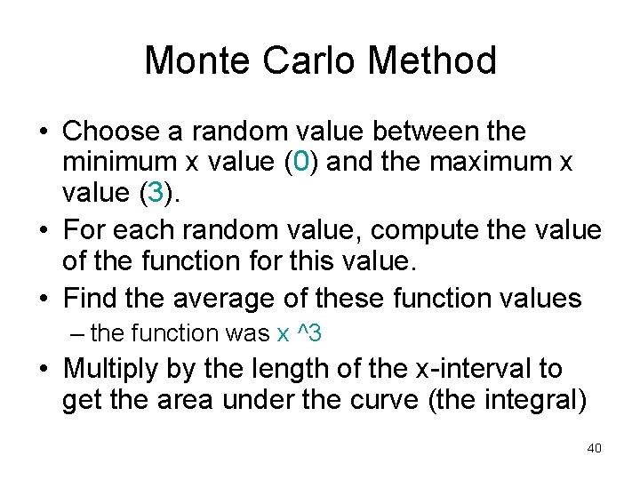
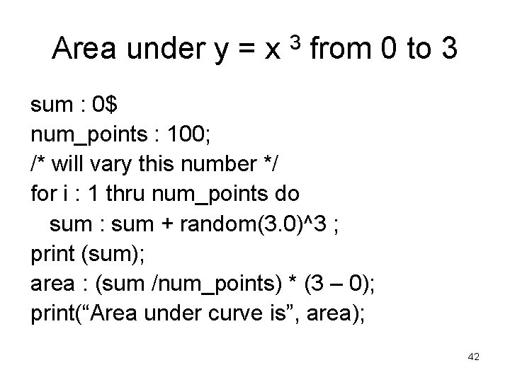
Monte Carlo Method • Choose a random value between the minimum x value (0) and the maximum x value (3). • For each random value, compute the value of the function for this value. • Find the average of these function values – the function was x ^3 • Multiply by the length of the x-interval to get the area under the curve (the integral) 40

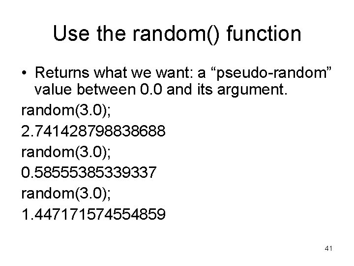
Use the random() function • Returns what we want: a “pseudo-random” value between 0. 0 and its argument. random(3. 0); 2. 741428798838688 random(3. 0); 0. 58555385339337 random(3. 0); 1. 447171574554859 41

Area under y = x 3 from 0 to 3 sum : 0$ num_points : 100; /* will vary this number */ for i : 1 thru num_points do sum : sum + random(3. 0)^3 ; print (sum); area : (sum /num_points) * (3 – 0); print(“Area under curve is”, area); 42

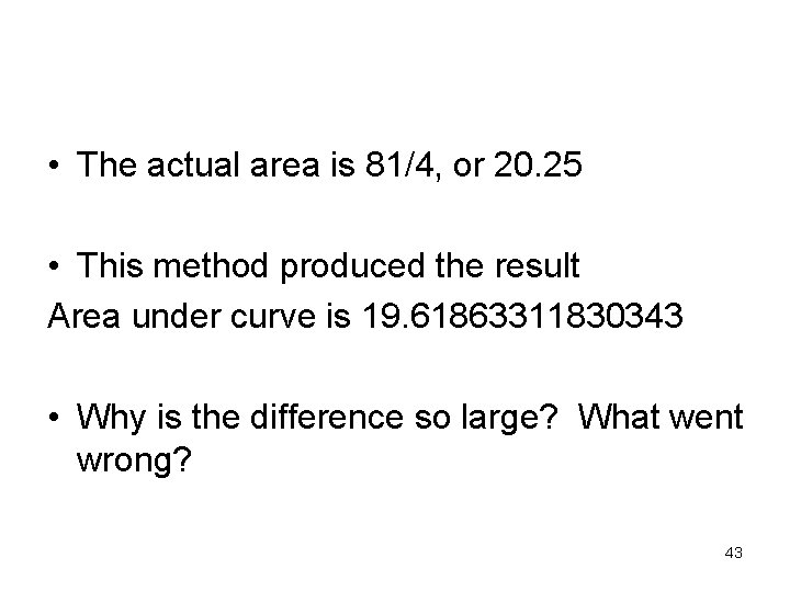
• The actual area is 81/4, or 20. 25 • This method produced the result Area under curve is 19. 61863311830343 • Why is the difference so large? What went wrong? 43

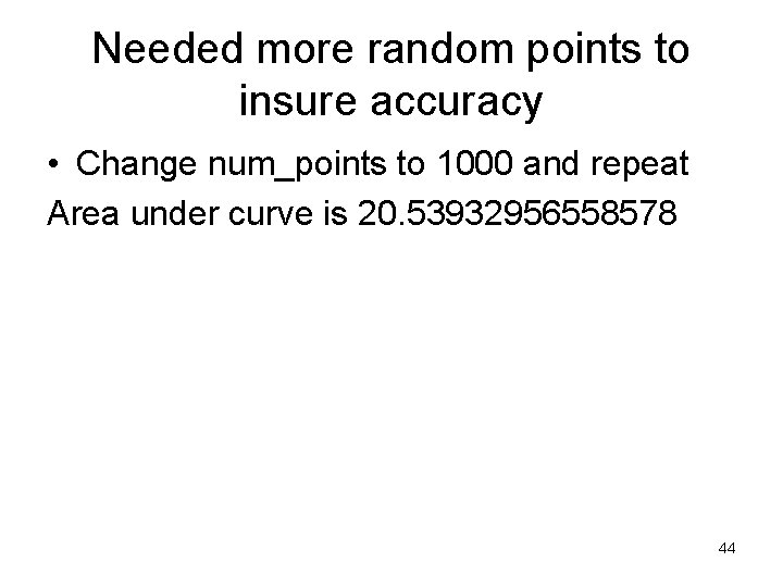
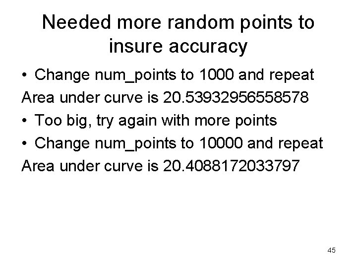
Needed more random points to insure accuracy • Change num_points to 1000 and repeat Area under curve is 20. 53932956558578 44

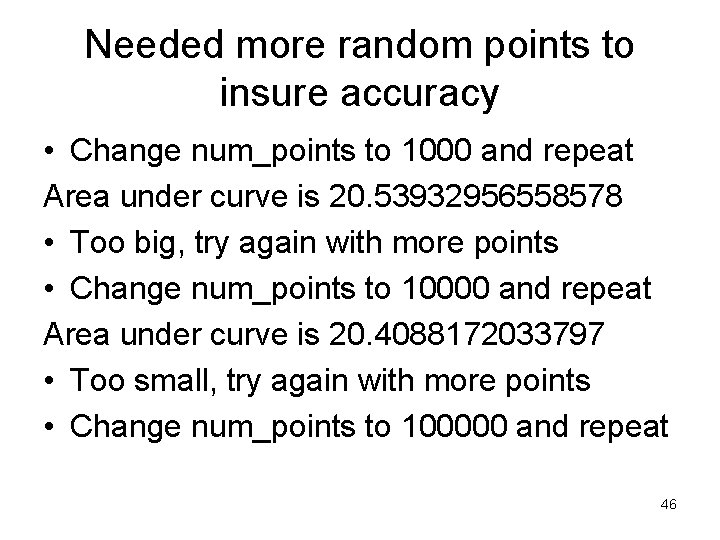
Needed more random points to insure accuracy • Change num_points to 1000 and repeat Area under curve is 20. 53932956558578 • Too big, try again with more points • Change num_points to 10000 and repeat Area under curve is 20. 4088172033797 45

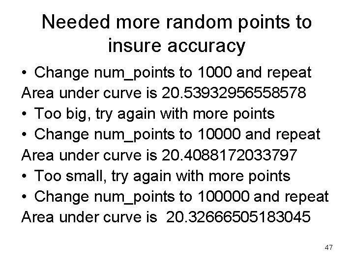
Needed more random points to insure accuracy • Change num_points to 1000 and repeat Area under curve is 20. 53932956558578 • Too big, try again with more points • Change num_points to 10000 and repeat Area under curve is 20. 4088172033797 • Too small, try again with more points • Change num_points to 100000 and repeat 46

Needed more random points to insure accuracy • Change num_points to 1000 and repeat Area under curve is 20. 53932956558578 • Too big, try again with more points • Change num_points to 10000 and repeat Area under curve is 20. 4088172033797 • Too small, try again with more points • Change num_points to 100000 and repeat Area under curve is 20. 32666505183045 47

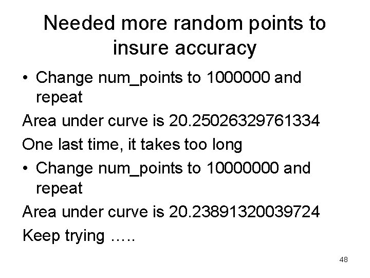
Needed more random points to insure accuracy • Change num_points to 1000000 and repeat Area under curve is 20. 25026329761334 One last time, it takes too long • Change num_points to 10000000 and repeat Area under curve is 20. 23891320039724 Keep trying …. . 48

Calculus of Several Variables 49

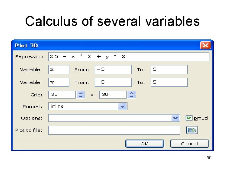
Calculus of several variables 50

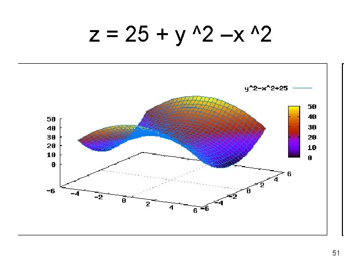
z = 25 + y ^2 –x ^2 51

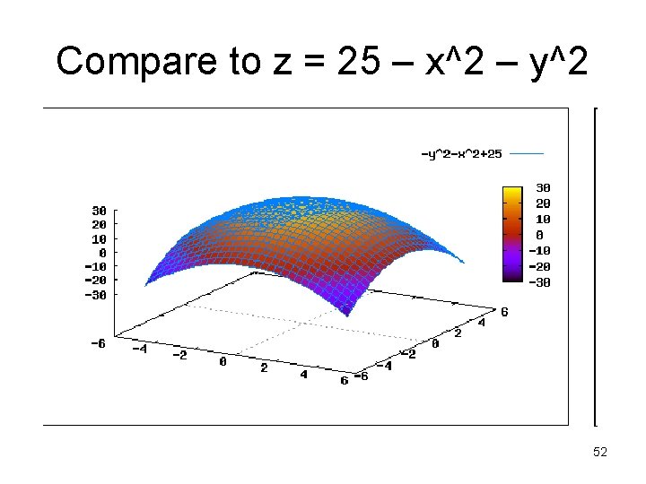
Compare to z = 25 – x^2 – y^2 52

Critical points • We saw the function f(x, y): = x * y ^2 + x *y; have partial derivatives y 2 + y and 2 xy+x 53

For critical points, both derivatives must be zero 54

Maxima solves systems solve([%o 12, %o 14], [x, y]); [ [x=0, y=0], [x=0, y=-1] ] 55