Sorting II Slide 1 Sorting l Arrange keys

Sorting II/ Slide 1 Sorting l Arrange keys in ascending or descending order. One of the most fundamental problems. First computer program was a sorting program (ENIAC, Univ. of Penn. ) l Studied: selection sort, insertion sort, merge sort (? ) and heap sort l

Sorting II/ Slide 2 Recall two basic sorting algorithms: l selection sorting l insertion sorting We will revisit the applet at: http: //math. hws. edu/TMCM/java/x. Sort. Lab/

Sorting II/ Slide 3 Merge sorting In lecture 2, we studied the merging step. Merging: Take two sorted arrays and combine them into one sorted array. Merge sorting and heap sorting are two algorithms that take O(n log n) time in the worst-case. (best possible)

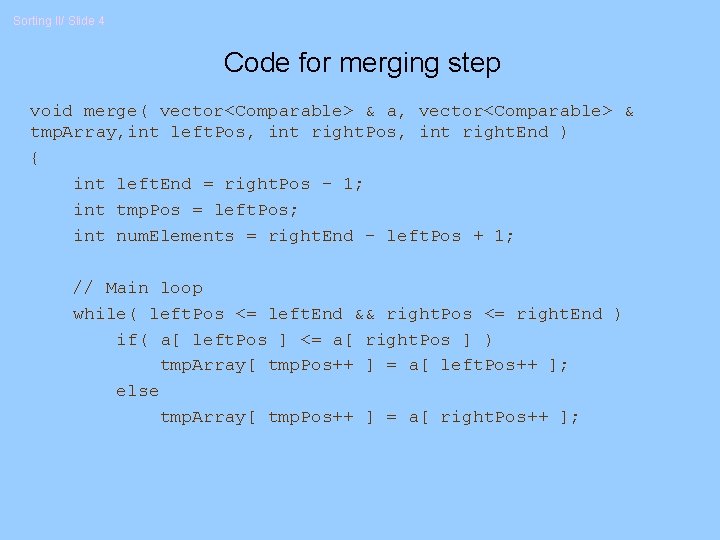
Sorting II/ Slide 4 Code for merging step void merge( vector<Comparable> & a, vector<Comparable> & tmp. Array, int left. Pos, int right. End ) { int left. End = right. Pos - 1; int tmp. Pos = left. Pos; int num. Elements = right. End - left. Pos + 1; // Main loop while( left. Pos <= left. End && right. Pos <= right. End ) if( a[ left. Pos ] <= a[ right. Pos ] ) tmp. Array[ tmp. Pos++ ] = a[ left. Pos++ ]; else tmp. Array[ tmp. Pos++ ] = a[ right. Pos++ ];

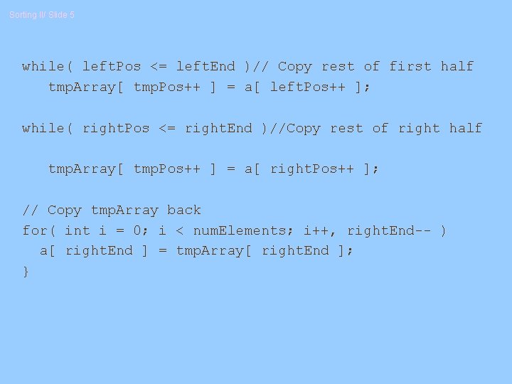
Sorting II/ Slide 5 while( left. Pos <= left. End )// Copy rest of first half tmp. Array[ tmp. Pos++ ] = a[ left. Pos++ ]; while( right. Pos <= right. End )//Copy rest of right half tmp. Array[ tmp. Pos++ ] = a[ right. Pos++ ]; // Copy tmp. Array back for( int i = 0; i < num. Elements; i++, right. End-- ) a[ right. End ] = tmp. Array[ right. End ]; }

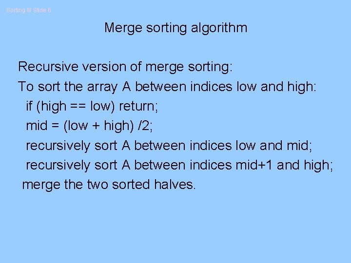
Sorting II/ Slide 6 Merge sorting algorithm Recursive version of merge sorting: To sort the array A between indices low and high: if (high == low) return; mid = (low + high) /2; recursively sort A between indices low and mid; recursively sort A between indices mid+1 and high; merge the two sorted halves.

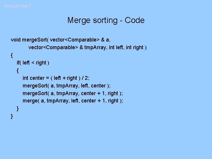
Sorting II/ Slide 7 Merge sorting - Code void merge. Sort( vector<Comparable> & a, vector<Comparable> & tmp. Array, int left, int right ) { if( left < right ) { int center = ( left + right ) / 2; merge. Sort( a, tmp. Array, left, center ); merge. Sort( a, tmp. Array, center + 1, right ); merge( a, tmp. Array, left, center + 1, right ); } }

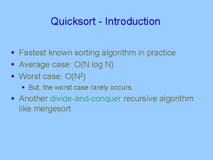
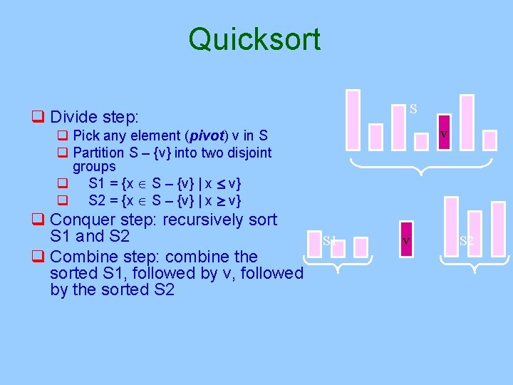
Quicksort - Introduction § Fastest known sorting algorithm in practice § Average case: O(N log N) § Worst case: O(N 2) § But, the worst case rarely occurs. § Another divide-and-conquer recursive algorithm like mergesort

Quicksort S q Divide step: v q Pick any element (pivot) v in S q Partition S – {v} into two disjoint groups q S 1 = {x S – {v} | x v} q S 2 = {x S – {v} | x v} q Conquer step: recursively sort S 1 and S 2 q Combine step: combine the sorted S 1, followed by v, followed by the sorted S 2 S 1 v S 2

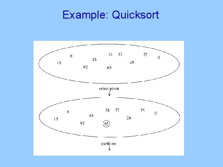
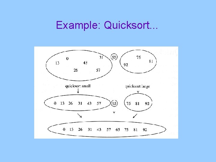
Example: Quicksort

Example: Quicksort. . .

Pseudocode Input: an array A[p, r] Quicksort (A, p, r) { if (p < r) { q = Partition (A, p, r) //q is the position of the pivot element Quicksort (A, p, q-1) Quicksort (A, q+1, r) } }

Partitioning § Partitioning Key step of quicksort algorithm § Goal: given the picked pivot, partition the remaining elements into two smaller sets § Many ways to implement § Even the slightest deviations may cause surprisingly bad results. § § § We will learn an easy and efficient partitioning strategy here. How to pick a pivot will be discussed later

Partitioning Strategy § § § Want to partition an array A[left. . right] First, get the pivot element out of the way by swapping it with the last element. (Swap pivot and A[right]) Let i start at the first element and j start at the next-tolast element (i = left, j = right – 1) swap 5 6 4 6 pivot 3 12 19 5 i 6 4 19 3 12 j 6

Partitioning Strategy § § Want to have § A[p] <= pivot, for p < i § A[p] >= pivot, for p > j When i < j § Move i right, skipping over elements smaller than the pivot § Move j left, skipping over elements greater than the pivot § When both i and j have stopped § A[i] >= pivot A[j]19<= 3 pivot 12 6 5 6§ 4 5 6 4 19 3 12 6 i j

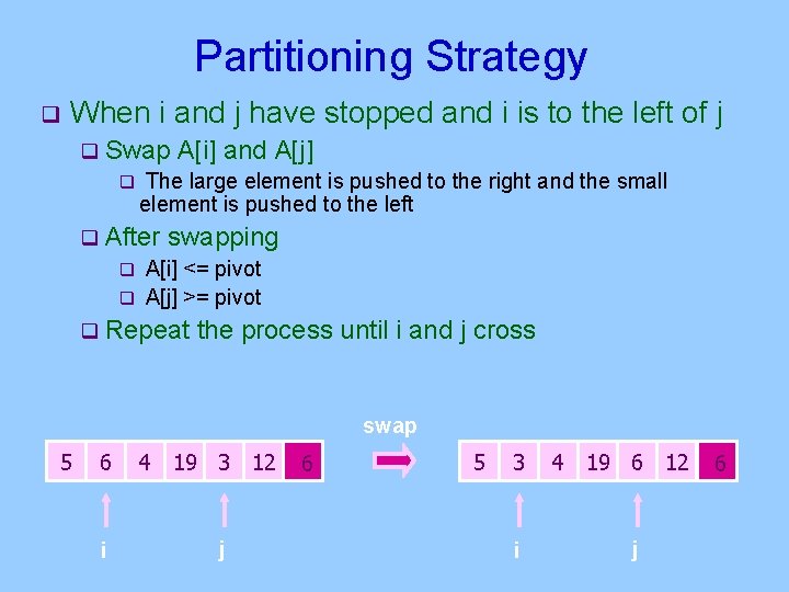
Partitioning Strategy q When i and j have stopped and i is to the left of j q Swap A[i] and A[j] q The large element is pushed to the right and the small element is pushed to the left q After swapping q A[i] <= pivot q A[j] >= pivot q Repeat the process until i and j cross swap 5 6 i 4 19 3 12 j 6 5 3 i 4 19 6 12 j 6

Partitioning Strategy q When i and j have crossed 5 q Swap A[i] and pivot q Result: q A[p] <= pivot, for p < i q A[p] >= pivot, for p > i 4 19 6 12 5 3 3 6 j i 5 http: //math. hws. edu/TMCM/java/x. Sort. Lab/ 3 4 19 6 12 j i 4 6 j i 6 6 12 19

Implementation of partitioning step int partition(A, left, right){ int pivot = A[right]; int i = left, j = right-1; for (; ; ) { while (a[i] < pivot && i <= right) i++; while (pivot < a[j] && j >= left) j--; if (i < j) {swap(a[i], a[j]); i++; j--; } else break; } swap(A[i], A[right]); return i; }

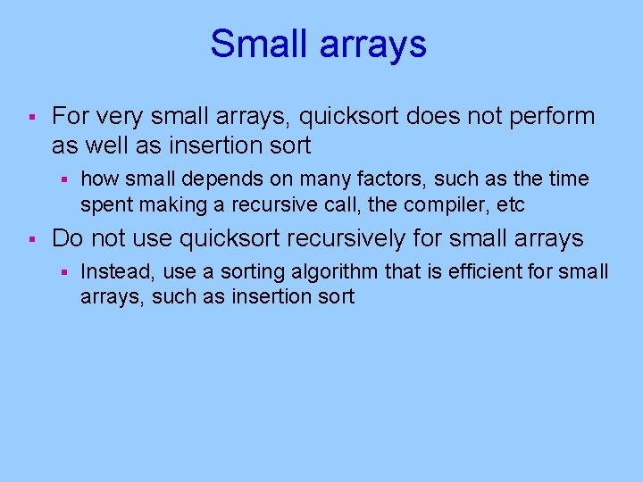
Small arrays § For very small arrays, quicksort does not perform as well as insertion sort § § how small depends on many factors, such as the time spent making a recursive call, the compiler, etc Do not use quicksort recursively for small arrays § Instead, use a sorting algorithm that is efficient for small arrays, such as insertion sort

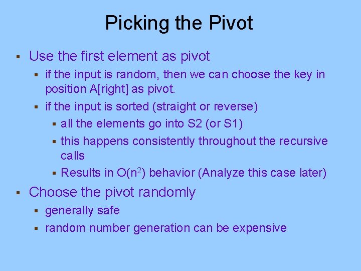
Picking the Pivot § Use the first element as pivot if the input is random, then we can choose the key in position A[right] as pivot. § if the input is sorted (straight or reverse) § all the elements go into S 2 (or S 1) § this happens consistently throughout the recursive calls § Results in O(n 2) behavior (Analyze this case later) § § Choose the pivot randomly generally safe § random number generation can be expensive §

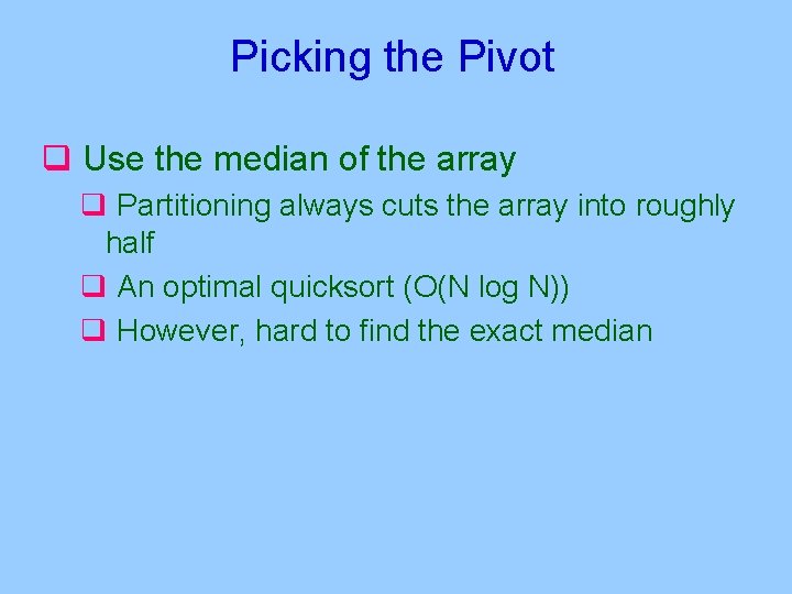
Picking the Pivot q Use the median of the array q Partitioning always cuts the array into roughly half q An optimal quicksort (O(N log N)) q However, hard to find the exact median

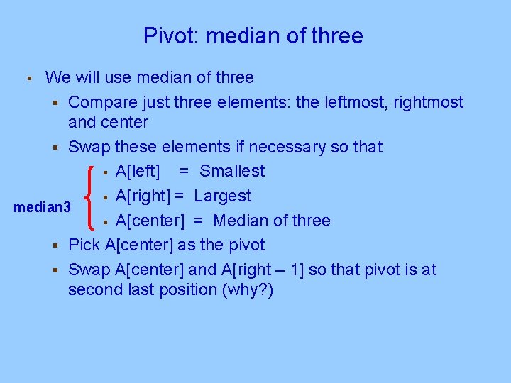
Pivot: median of three We will use median of three § Compare just three elements: the leftmost, rightmost and center § Swap these elements if necessary so that § A[left] = Smallest § A[right] = Largest median 3 § A[center] = Median of three § Pick A[center] as the pivot § Swap A[center] and A[right – 1] so that pivot is at second last position (why? ) §

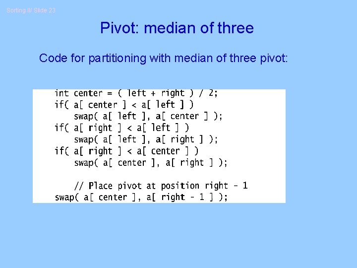
Sorting II/ Slide 23 Pivot: median of three Code for partitioning with median of three pivot:

Pivot: median of three A[left] = 2, A[center] = 13, A[right] = 6 2 5 6 4 13 3 12 19 2 5 6 4 6 3 12 19 13 Swap A[center] and A[right] 2 5 6 4 6 3 12 19 13 Choose A[center] as pivot 6 pivot 2 5 6 4 19 3 12 6 13 Swap pivot and A[right – 1] pivot Note we only need to partition A[left + 1, …, right – 2]. Why?

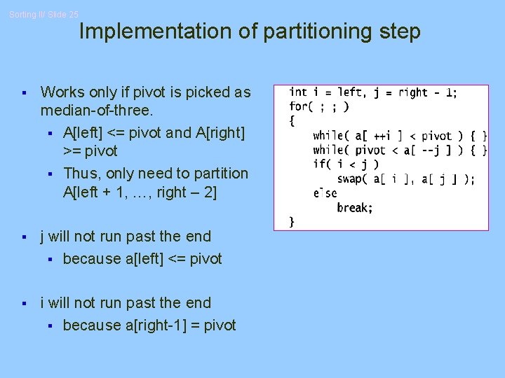
Sorting II/ Slide 25 Implementation of partitioning step § Works only if pivot is picked as median-of-three. § A[left] <= pivot and A[right] >= pivot § Thus, only need to partition A[left + 1, …, right – 2] § j will not run past the end § because a[left] <= pivot § i will not run past the end § because a[right-1] = pivot

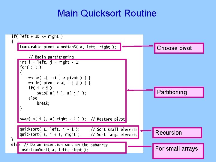
Main Quicksort Routine Choose pivot Partitioning Recursion For small arrays

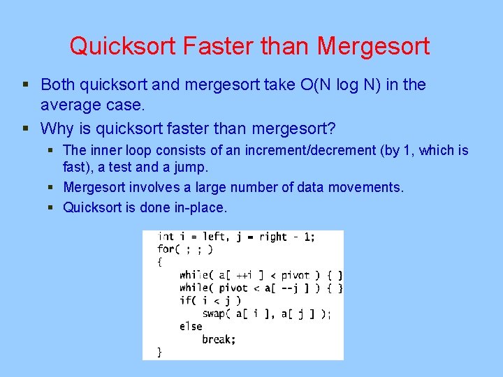
Quicksort Faster than Mergesort § Both quicksort and mergesort take O(N log N) in the average case. § Why is quicksort faster than mergesort? § The inner loop consists of an increment/decrement (by 1, which is fast), a test and a jump. § Mergesort involves a large number of data movements. § Quicksort is done in-place.

Performance of quicksort § § Worst-case: takes O(n 2) time. Average-case: takes O(n log n) time. On typical inputs, quicksort runs faster than other algorithms. Compare various sorting algorithms at: http: //www. geocities. com/siliconvalley/network/1854/ Sort 1. html