Sorting Algorithms Sorting Its a way to arrange
![Bubble Sort Illustration Iteration 1: a[0] a[1] a[2] a[3] a[4] a[5] a[6] a[7] a[8] Bubble Sort Illustration Iteration 1: a[0] a[1] a[2] a[3] a[4] a[5] a[6] a[7] a[8]](https://slidetodoc.com/presentation_image_h2/4856895c634aa23d7901ea73fa82bc9d/image-5.jpg)
![a[0] a[1] a[2] a[3] a[4] a[5] a[6] a[7] a[8] a[9] 7 5 7 2 a[0] a[1] a[2] a[3] a[4] a[5] a[6] a[7] a[8] a[9] 7 5 7 2](https://slidetodoc.com/presentation_image_h2/4856895c634aa23d7901ea73fa82bc9d/image-6.jpg)
![Selection Sort Illustration Iteration 1: a[0] a[1] a[2] a[3] a[4] a[5] a[6] a[7] a[8] Selection Sort Illustration Iteration 1: a[0] a[1] a[2] a[3] a[4] a[5] a[6] a[7] a[8]](https://slidetodoc.com/presentation_image_h2/4856895c634aa23d7901ea73fa82bc9d/image-13.jpg)
![a[0] a[1] a[2] a[3] a[4] a[5] a[6] a[7] a[8] a[9] 2 7 7 13 a[0] a[1] a[2] a[3] a[4] a[5] a[6] a[7] a[8] a[9] 2 7 7 13](https://slidetodoc.com/presentation_image_h2/4856895c634aa23d7901ea73fa82bc9d/image-14.jpg)
![Insertion Sort Illustration Pass 1: a[0] a[1] a[2] a[3] a[4] a[5] a[6] a[7] a[8] Insertion Sort Illustration Pass 1: a[0] a[1] a[2] a[3] a[4] a[5] a[6] a[7] a[8]](https://slidetodoc.com/presentation_image_h2/4856895c634aa23d7901ea73fa82bc9d/image-21.jpg)
![Quick Sort Illustration left right 4 6 low high pivot = A[low] left 8 Quick Sort Illustration left right 4 6 low high pivot = A[low] left 8](https://slidetodoc.com/presentation_image_h2/4856895c634aa23d7901ea73fa82bc9d/image-40.jpg)
- Slides: 77

Sorting Algorithms

Sorting Ø It’s a way to arrange the unordered collection in some order like ascending or descending Types of sorting algorithms – 1. Bubble Sort 2. Selection Sort 3. Insertion Sort 4. Quick Sort 5. Merge Sort 6. Heap Sort 7. Radix Sort 8. Shell Sort etc.

Internal and External Sorting ØInternal sort is any data sorting process that takes place entirely within the main memory of a computer. • This is possible whenever the data to be sorted is small enough to all be held in the main memory. ØExternal sorting is a term for a class of sorting algorithms that can handle massive amounts of data. • External sorting is required when the data being sorted do not fit into the main memory of a computing device (usually RAM) and instead they must reside in the slower external memory (usually a hard drive). External merge sort One example of external sorting is the external merge sort algorithm, which sorts chunks that each fit in RAM, then merges the sorted chunks together. For example, for sorting 900 megabytes of data using only 100 megabytes of RAM

Bubble Sort Ø Move from left to right end Ø Compare the two elements and swap them if needed
![Bubble Sort Illustration Iteration 1 a0 a1 a2 a3 a4 a5 a6 a7 a8 Bubble Sort Illustration Iteration 1: a[0] a[1] a[2] a[3] a[4] a[5] a[6] a[7] a[8]](https://slidetodoc.com/presentation_image_h2/4856895c634aa23d7901ea73fa82bc9d/image-5.jpg)
Bubble Sort Illustration Iteration 1: a[0] a[1] a[2] a[3] a[4] a[5] a[6] a[7] a[8] a[9] 7 7 5 13 2 3 9 3 1 0 No Swapping 7 7 5 13 2 3 9 3 1 0 Swapping 7 5 7 13 2 3 9 3 1 0 No Swapping 7 5 7 13 2 3 9 3 1 0 Swapping 7 5 7 2 13 3 9 3 1 0 Swapping 7 5 7 2 3 13 9 3 1 0 Swapping 7 5 7 2 3 9 13 3 1 0 Swapping
![a0 a1 a2 a3 a4 a5 a6 a7 a8 a9 7 5 7 2 a[0] a[1] a[2] a[3] a[4] a[5] a[6] a[7] a[8] a[9] 7 5 7 2](https://slidetodoc.com/presentation_image_h2/4856895c634aa23d7901ea73fa82bc9d/image-6.jpg)
a[0] a[1] a[2] a[3] a[4] a[5] a[6] a[7] a[8] a[9] 7 5 7 2 3 9 3 13 1 0 Swapping 7 5 7 2 3 9 3 1 13 0 Swapping 7 5 7 2 3 9 3 1 0 13 Swapping Final Position Iteration 2: 5 7 2 3 7 3 1 0 9 13 Final Position

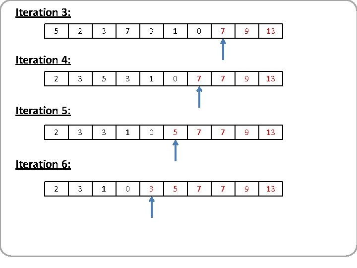
Iteration 3: 5 2 3 7 3 1 0 7 9 13 3 5 3 1 0 7 7 9 13 3 3 1 0 5 7 7 9 13 3 1 0 3 5 7 7 9 13 Iteration 4: 2 Iteration 5: 2 Iteration 6: 2

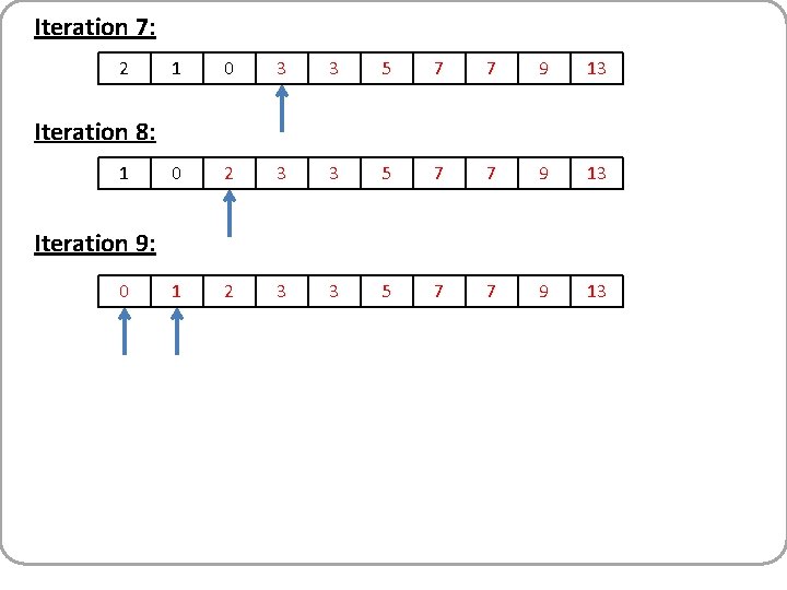
Iteration 7: 2 1 0 3 3 5 7 7 9 13 0 2 3 3 5 7 7 9 13 1 2 3 3 5 7 7 9 13 Iteration 8: 1 Iteration 9: 0

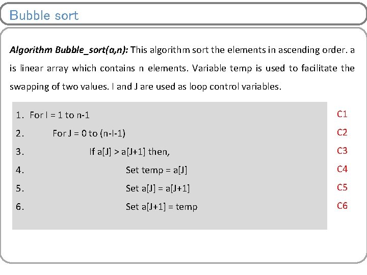
Bubble sort Algorithm Bubble_sort(a, n): This algorithm sort the elements in ascending order. a is linear array which contains n elements. Variable temp is used to facilitate the swapping of two values. I and J are used as loop control variables. 1. For I = 1 to n-1 C 1 2. C 2 3. For J = 0 to (n-I-1) If a[J] > a[J+1] then, C 3 4. Set temp = a[J] C 4 5. Set a[J] = a[J+1] C 5 6. Set a[J+1] = temp C 6

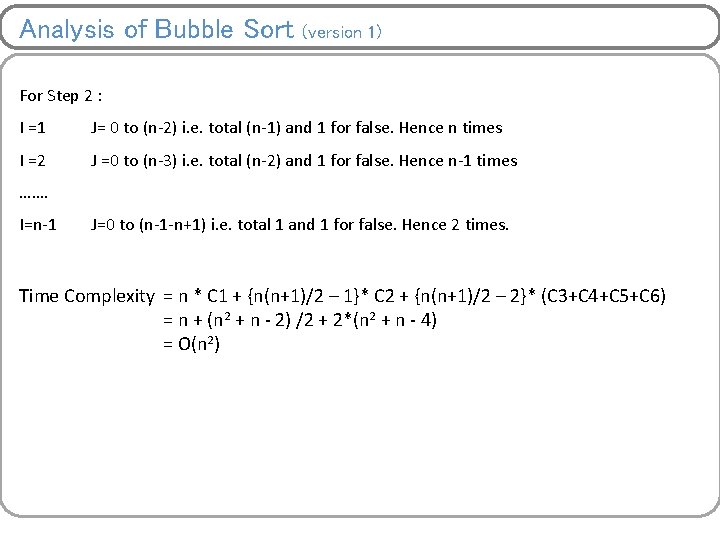
Analysis of Bubble Sort (version 1) For Step 2 : I =1 J= 0 to (n-2) i. e. total (n-1) and 1 for false. Hence n times I =2 J =0 to (n-3) i. e. total (n-2) and 1 for false. Hence n-1 times ……. I=n-1 J=0 to (n-1 -n+1) i. e. total 1 and 1 for false. Hence 2 times. Time Complexity = n * C 1 + {n(n+1)/2 – 1}* C 2 + {n(n+1)/2 – 2}* (C 3+C 4+C 5+C 6) = n + (n 2 + n - 2) /2 + 2*(n 2 + n - 4) = O(n 2)

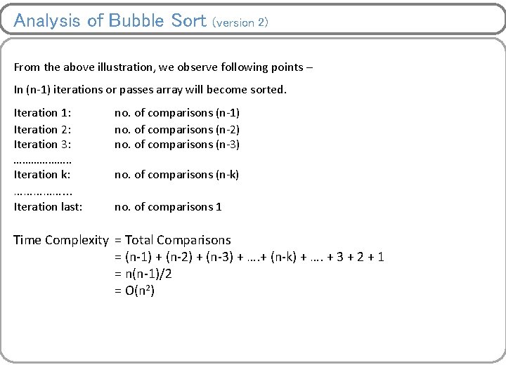
Analysis of Bubble Sort (version 2) From the above illustration, we observe following points – In (n-1) iterations or passes array will become sorted. Iteration 1: Iteration 2: Iteration 3: ………………. . Iteration k: no. of comparisons (n-1) no. of comparisons (n-2) no. of comparisons (n-3) Iteration last: no. of comparisons 1 ……………. . . no. of comparisons (n-k) Time Complexity = Total Comparisons = (n-1) + (n-2) + (n-3) + …. + (n-k) + …. + 3 + 2 + 1 = n(n-1)/2 = O(n 2)

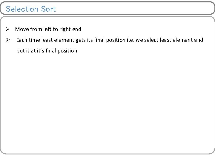
Selection Sort Ø Move from left to right end Ø Each time least element gets its final position i. e. we select least element and put it at it’s final position
![Selection Sort Illustration Iteration 1 a0 a1 a2 a3 a4 a5 a6 a7 a8 Selection Sort Illustration Iteration 1: a[0] a[1] a[2] a[3] a[4] a[5] a[6] a[7] a[8]](https://slidetodoc.com/presentation_image_h2/4856895c634aa23d7901ea73fa82bc9d/image-13.jpg)
Selection Sort Illustration Iteration 1: a[0] a[1] a[2] a[3] a[4] a[5] a[6] a[7] a[8] a[9] 7 7 5 13 2 3 9 3 1 0 No Swapping 7 7 5 13 2 3 9 3 1 0 Swapping 5 7 7 13 2 3 9 3 1 0 No Swapping 5 7 7 13 2 3 9 3 1 0 Swapping 2 7 7 13 5 3 9 3 1 0 No Swapping
![a0 a1 a2 a3 a4 a5 a6 a7 a8 a9 2 7 7 13 a[0] a[1] a[2] a[3] a[4] a[5] a[6] a[7] a[8] a[9] 2 7 7 13](https://slidetodoc.com/presentation_image_h2/4856895c634aa23d7901ea73fa82bc9d/image-14.jpg)
a[0] a[1] a[2] a[3] a[4] a[5] a[6] a[7] a[8] a[9] 2 7 7 13 5 3 9 3 1 0 Swapping 1 7 7 13 5 3 9 3 2 0 Swapping 0 7 7 13 5 3 9 3 2 1 7 13 7 5 9 3 3 2 Final Position Iteration 2: 0 1 Final Position

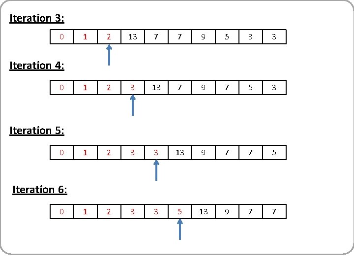
Iteration 3: 0 1 2 13 7 7 9 5 3 3 1 2 3 13 7 9 7 5 3 1 2 3 3 13 9 7 7 5 1 2 3 3 5 13 9 7 7 Iteration 4: 0 Iteration 5: 0 Iteration 6: 0

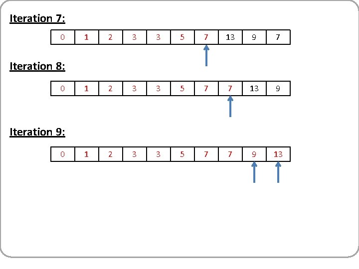
Iteration 7: 0 1 2 3 3 5 7 13 9 7 1 2 3 3 5 7 7 13 9 1 2 3 3 5 7 7 9 13 Iteration 8: 0 Iteration 9: 0

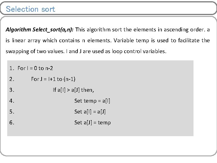
Selection sort Algorithm Select_sort(a, n): This algorithm sort the elements in ascending order. a is linear array which contains n elements. Variable temp is used to facilitate the swapping of two values. I and J are used as loop control variables. 1. For I = 0 to n-2 2. 3. For J = I+1 to (n-1) If a[I] > a[J] then, 4. Set temp = a[I] 5. Set a[I] = a[J] 6. Set a[J] = temp

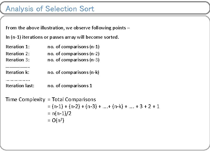
Analysis of Selection Sort From the above illustration, we observe following points – In (n-1) iterations or passes array will become sorted. Iteration 1: Iteration 2: Iteration 3: ………………. . Iteration k: no. of comparisons (n-1) no. of comparisons (n-2) no. of comparisons (n-3) Iteration last: no. of comparisons 1 ……………. . . no. of comparisons (n-k) Time Complexity = Total Comparisons = (n-1) + (n-2) + (n-3) + …. + (n-k) + …. + 3 + 2 + 1 = n(n-1)/2 = O(n 2)

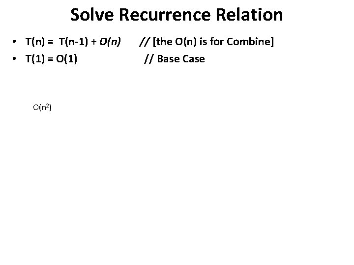
Solve Recurrence Relation • T(n) = T(n-1) + O(n) • T(1) = O(1) O(n 2) // [the O(n) is for Combine] // Base Case

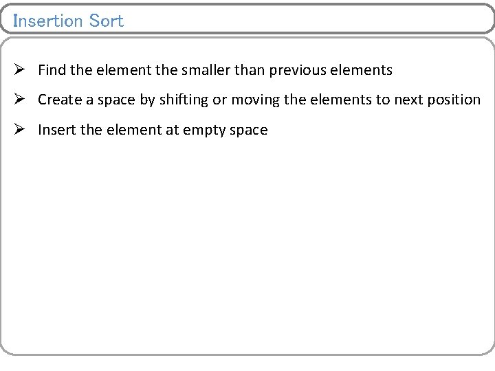
Insertion Sort Ø Find the element the smaller than previous elements Ø Create a space by shifting or moving the elements to next position Ø Insert the element at empty space
![Insertion Sort Illustration Pass 1 a0 a1 a2 a3 a4 a5 a6 a7 a8 Insertion Sort Illustration Pass 1: a[0] a[1] a[2] a[3] a[4] a[5] a[6] a[7] a[8]](https://slidetodoc.com/presentation_image_h2/4856895c634aa23d7901ea73fa82bc9d/image-21.jpg)
Insertion Sort Illustration Pass 1: a[0] a[1] a[2] a[3] a[4] a[5] a[6] a[7] a[8] a[9] 7 7 5 13 2 3 9 3 1 0 5 7 7 13 2 3 9 3 1 0 Pass 2: Pass 3:

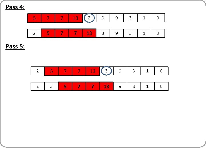
Pass 4: 5 7 7 13 2 3 9 3 1 0 2 5 7 7 13 3 9 3 1 0 Pass 5: 2 5 7 7 13 3 9 3 1 0 2 3 5 7 7 13 9 3 1 0

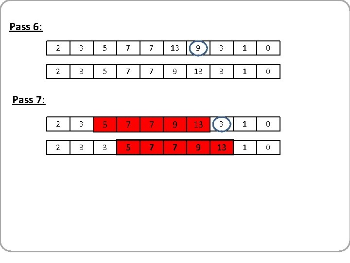
Pass 6: 2 3 5 7 7 13 9 3 1 0 2 3 5 7 7 9 13 3 1 0 2 3 3 5 7 7 9 13 1 0 Pass 7:

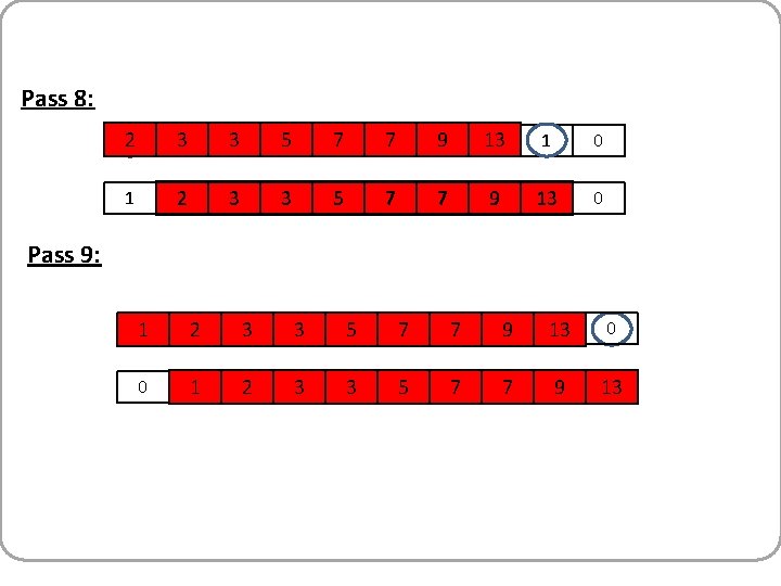
Pass 8: 2 3 3 5 7 7 9 13 1 0 1 2 3 3 5 7 7 9 13 0 Pass 9: 1 2 3 3 5 7 7 9 13 0 0 1 2 3 3 5 7 7 9 13

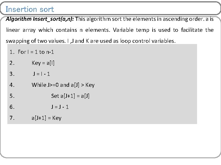
Insertion sort Algorithm Insert_sort(a, n): This algorithm sort the elements in ascending order. a is linear array which contains n elements. Variable temp is used to facilitate the swapping of two values. I , J and K are used as loop control variables. 1. For I = 1 to n-1 2. Key = a[I] 3. J=I-1 4. While J>=0 and a[J] > Key 5. Set a[J+1] = a[J] 6. J=J-1 7. a[J+1] = Key

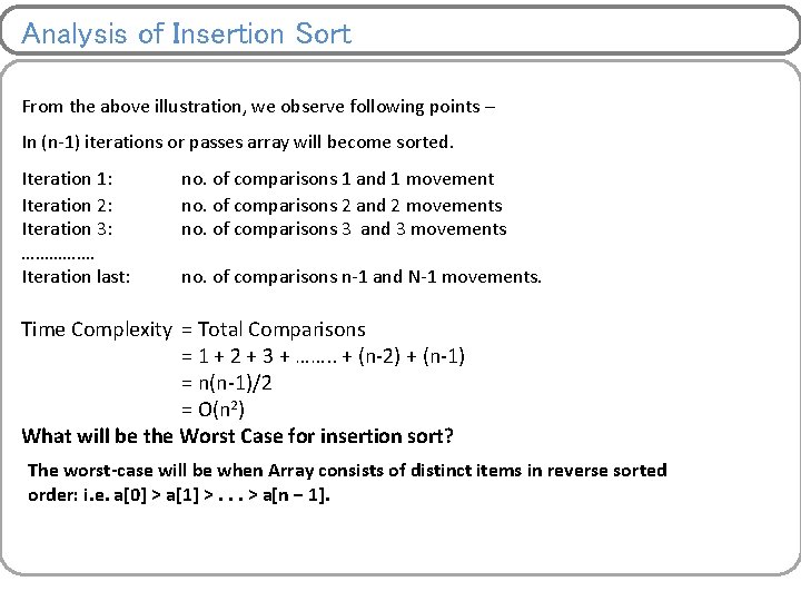
Analysis of Insertion Sort From the above illustration, we observe following points – In (n-1) iterations or passes array will become sorted. Iteration 1: Iteration 2: Iteration 3: ……………. Iteration last: no. of comparisons 1 and 1 movement no. of comparisons 2 and 2 movements no. of comparisons 3 and 3 movements no. of comparisons n-1 and N-1 movements. Time Complexity = Total Comparisons = 1 + 2 + 3 + ……. . + (n-2) + (n-1) = n(n-1)/2 = O(n 2) What will be the Worst Case for insertion sort? The worst-case will be when Array consists of distinct items in reverse sorted order: i. e. a[0] > a[1] >. . . > a[n − 1].

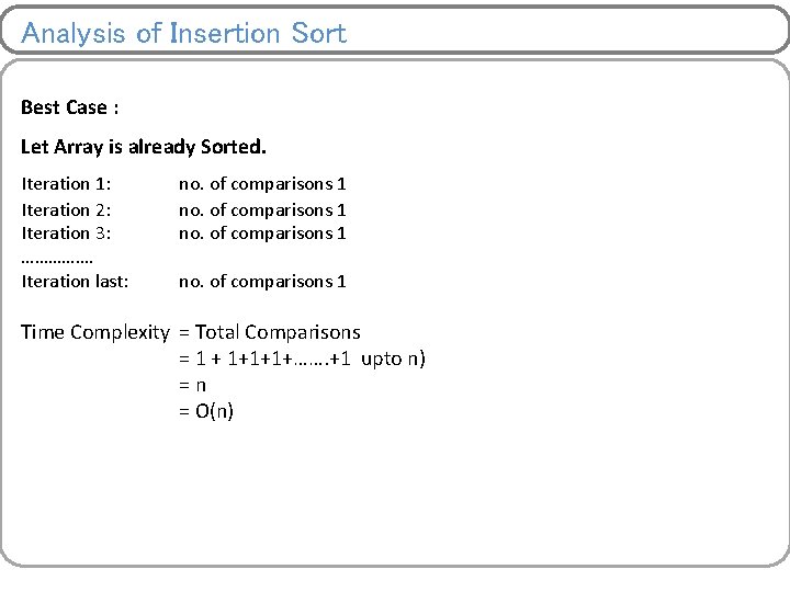
Analysis of Insertion Sort Best Case : Let Array is already Sorted. Iteration 1: Iteration 2: Iteration 3: ……………. Iteration last: no. of comparisons 1 Time Complexity = Total Comparisons = 1 + 1+1+1+……. +1 upto n) =n = O(n)

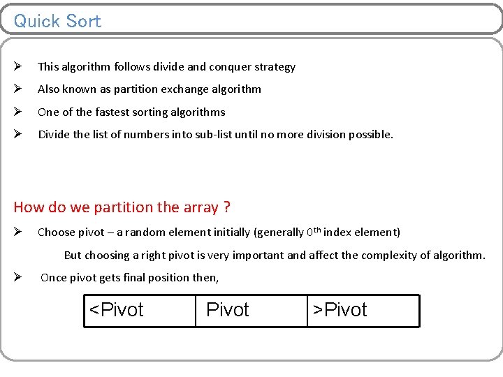
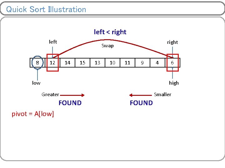
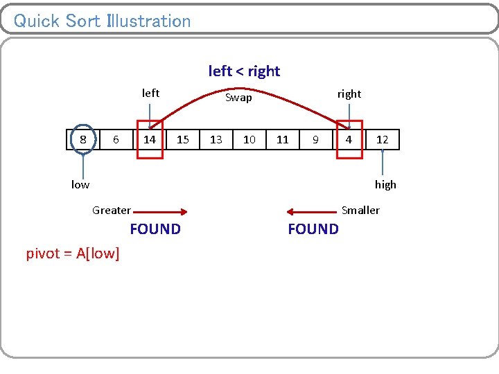
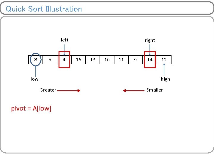
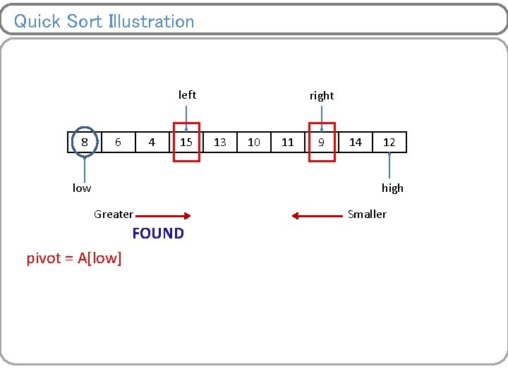
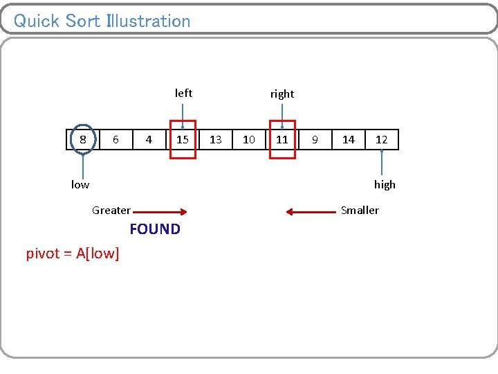
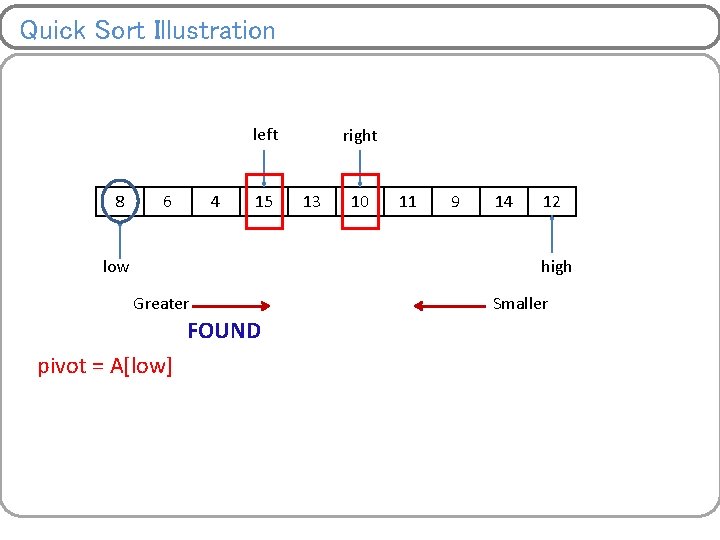
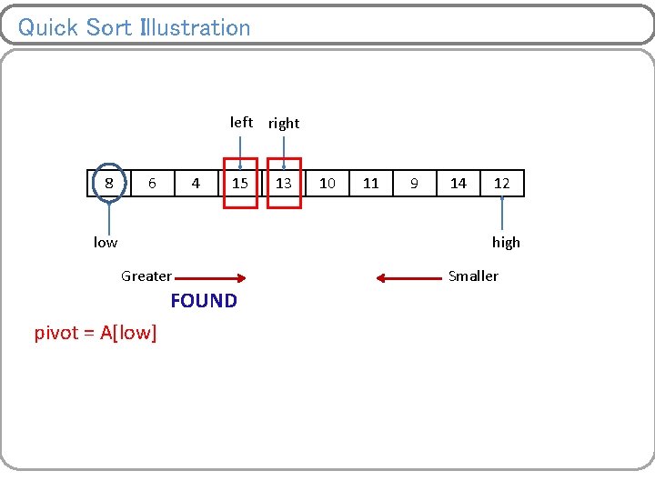
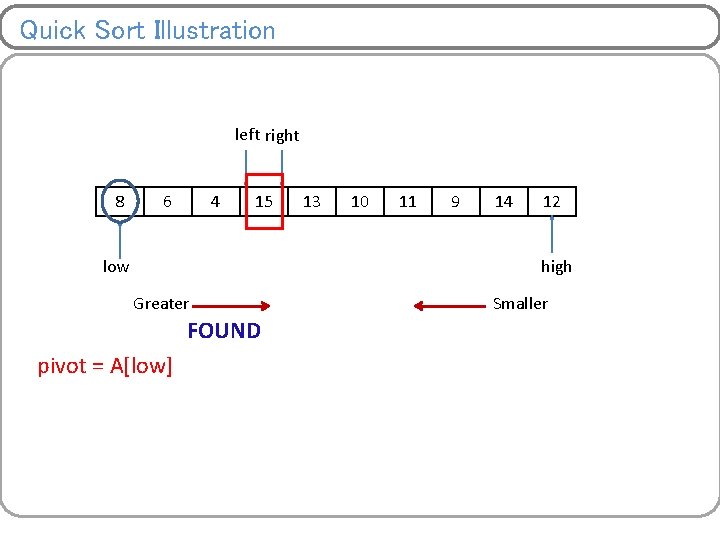
Quick Sort Ø This algorithm follows divide and conquer strategy Ø Also known as partition exchange algorithm Ø One of the fastest sorting algorithms Ø Divide the list of numbers into sub-list until no more division possible. How do we partition the array ? Ø Choose pivot – a random element initially (generally 0 th index element) But choosing a right pivot is very important and affect the complexity of algorithm. Ø Once pivot gets final position then, <Pivot >Pivot

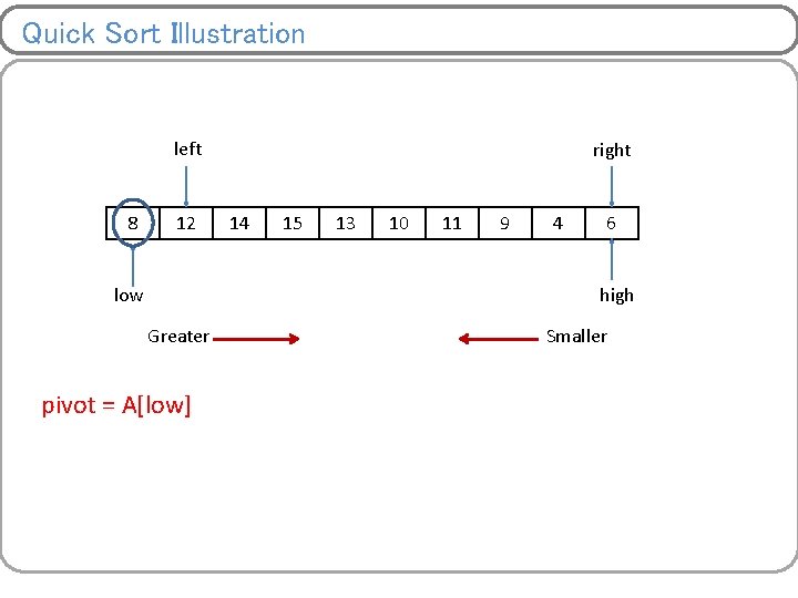
Quick Sort Illustration left 8 12 low right 14 15 13 10 11 9 4 6 high Greater pivot = A[low] Smaller

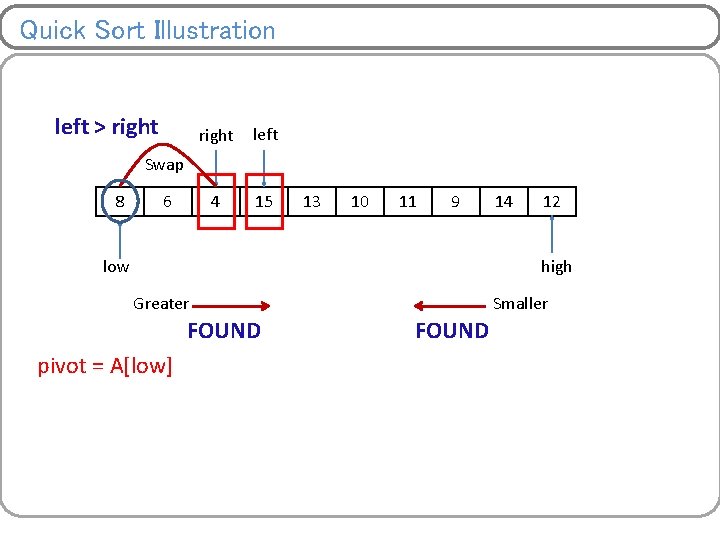
Quick Sort Illustration left < right left 8 right Swap 12 14 15 13 10 11 9 low 4 6 high Greater FOUND pivot = A[low] Smaller FOUND

Quick Sort Illustration left < right left 8 6 14 right Swap 15 13 10 11 9 low 4 12 high Greater FOUND pivot = A[low] Smaller FOUND

Quick Sort Illustration left 8 6 low 4 right 15 13 10 11 9 14 12 high Greater pivot = A[low] Smaller

Quick Sort Illustration left 8 6 4 15 low right 13 10 11 9 14 12 high Greater FOUND pivot = A[low] Smaller

Quick Sort Illustration left 8 6 4 15 low right 13 10 11 9 14 12 high Greater FOUND pivot = A[low] Smaller

Quick Sort Illustration left 8 6 4 15 low right 13 10 11 9 14 12 high Greater FOUND pivot = A[low] Smaller

Quick Sort Illustration left right 8 6 4 15 low 13 10 11 9 14 12 high Greater FOUND pivot = A[low] Smaller

Quick Sort Illustration left right 8 6 4 15 low 13 10 11 9 14 12 high Greater FOUND pivot = A[low] Smaller

Quick Sort Illustration left > right left 4 15 Swap 8 6 13 10 11 9 low 14 12 high Greater FOUND pivot = A[low] Smaller FOUND

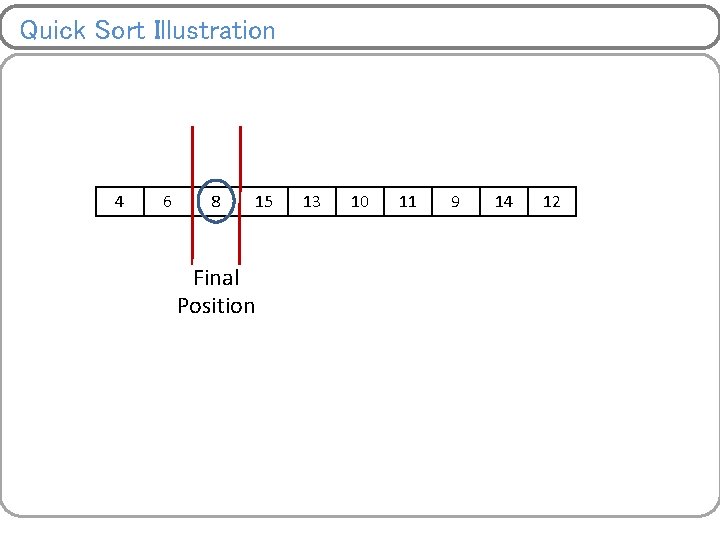
Quick Sort Illustration 4 6 8 15 Final Position 13 10 11 9 14 12
![Quick Sort Illustration left right 4 6 low high pivot Alow left 8 Quick Sort Illustration left right 4 6 low high pivot = A[low] left 8](https://slidetodoc.com/presentation_image_h2/4856895c634aa23d7901ea73fa82bc9d/image-40.jpg)
Quick Sort Illustration left right 4 6 low high pivot = A[low] left 8 15 low 13 right 10 11 9 14 12 high

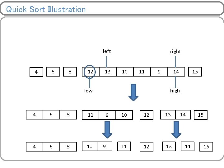
Quick Sort Illustration left 4 6 8 12 13 right 10 11 low 4 6 8 11 4 6 8 10 9 14 15 high 9 9 10 12 13 11 12 13 14 14 15 15

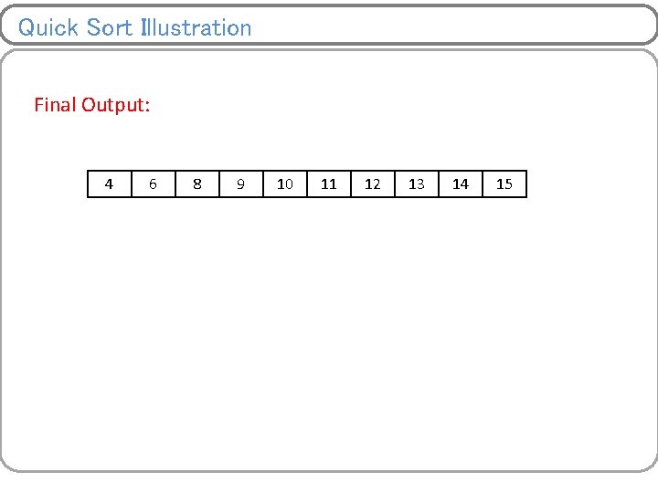
Quick Sort Illustration Final Output: 4 6 8 9 10 11 12 13 14 15

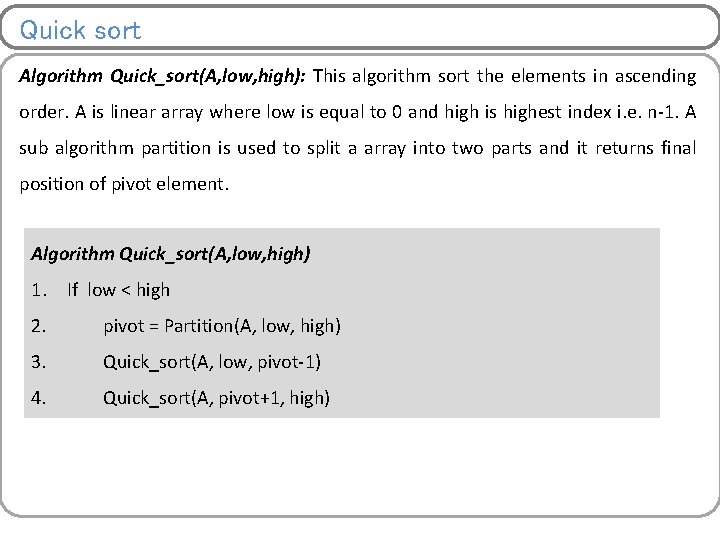
Quick sort Algorithm Quick_sort(A, low, high): This algorithm sort the elements in ascending order. A is linear array where low is equal to 0 and high is highest index i. e. n-1. A sub algorithm partition is used to split a array into two parts and it returns final position of pivot element. Algorithm Quick_sort(A, low, high) 1. If low < high 2. pivot = Partition(A, low, high) 3. Quick_sort(A, low, pivot-1) 4. Quick_sort(A, pivot+1, high)

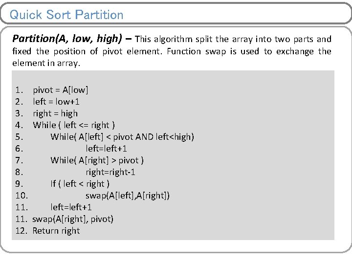
Quick Sort Partition(A, low, high) – This algorithm split the array into two parts and fixed the position of pivot element. Function swap is used to exchange the element in array. 1. 2. 3. 4. 5. 6. 7. 8. 9. 10. 11. 12. pivot = A[low] left = low+1 right = high While ( left <= right ) While( A[left] < pivot AND left<high) left=left+1 While( A[right] > pivot ) right=right-1 If ( left < right ) swap(A[left], A[right]) left=left+1 swap(A[right], pivot) Return right

Show all iteration of insertion Sort • 84, 69, 76, 86, 94, 91

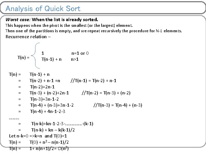
Analysis of Quick Sort Worst case: When the list is already sorted. This happens when the pivot is the smallest (or the largest) element. Then one of the partitions is empty, and we repeat recursively the procedure for N-1 elements. Recurrence relation – T(n) = 1 T(n-1) + n n=1 or 0 n>1 T(n) = T(n-1) + n = T(n-2) + n-1 +n //T(n-1) = T(n-2) + n-1 = T(n-2)+2 n-1 = T(n-3) + (n-2)+2 n-1 //T(n-2) = T(n-3) + (n-2) = T(n-3)+3 n-1 -2 = T(n-4) + (n-3)+3 n-1 -2 //T(n-3) = T(n-4) + 4 n-1 -2 -3. . . . = T(n-k)+kn-1 -2 -3 -. . . -(k-1) = T(n-k) + kn – k(k-1)/2 Let n-k=0 =>k=n and T(0)=1 T(n) = T(0) + n 2 – n(n-1)/2 T(n) = 1+ n(n+1)/2= O(n 2)

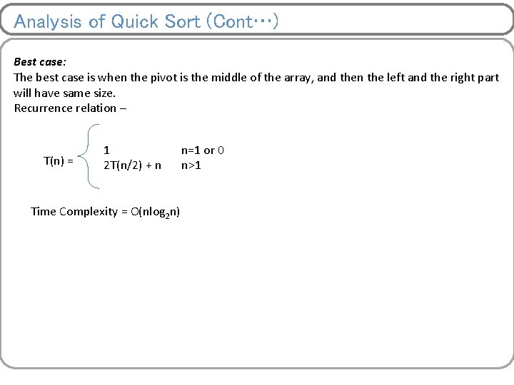
Analysis of Quick Sort (Cont…) Best case: The best case is when the pivot is the middle of the array, and then the left and the right part will have same size. Recurrence relation – T(n) = 1 2 T(n/2) + n Time Complexity = O(nlog 2 n) n=1 or 0 n>1

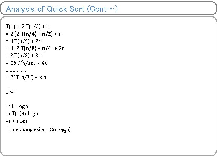
Analysis of Quick Sort (Cont…) T(n) = 2 T(n/2) + n = 2 [2 T(n/4) + n/2] + n = 4 T(n/4) + 2 n = 4 [2 T(n/8) + n/4] + 2 n = 8 T(n/8) + 3 n = 16 T(n/16) + 4 n …………… = 2 k T(n/2 k) + k n 2 k=n =>k=logn =n. T(1)+nlogn =n+nlogn Time Complexity = O(nlog 2 n)

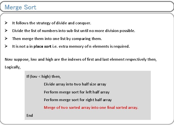
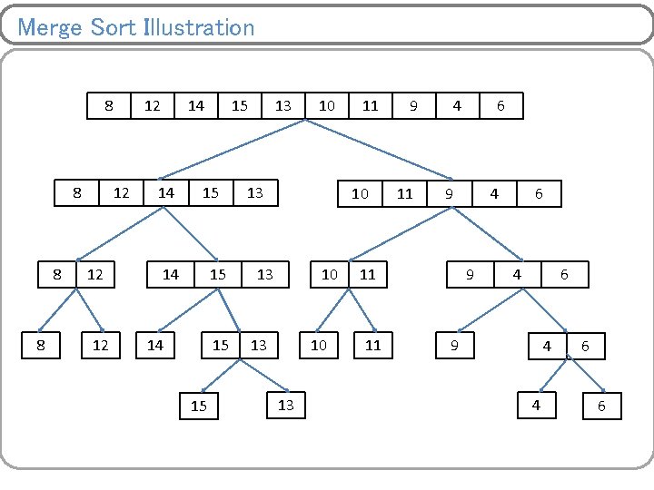
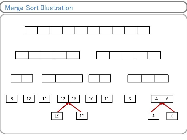
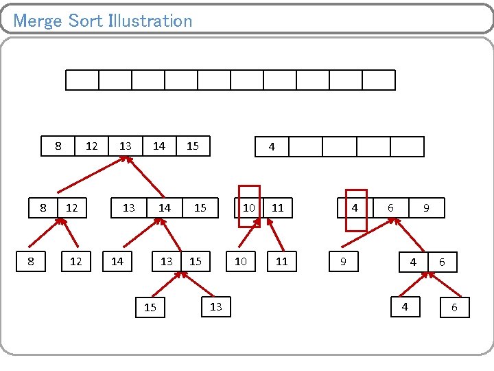
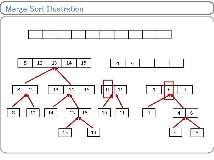
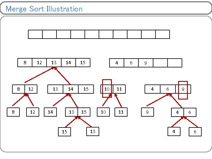
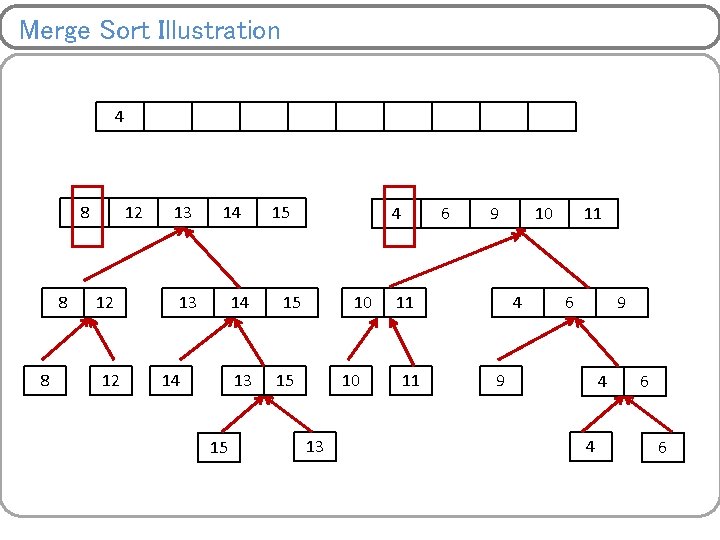
Merge Sort Ø It follows the strategy of divide and conquer. Ø Divide the list of numbers into sub-list until no more division possible. Ø Then merge them into one list by comparing them. Ø It is not a in place sort i. e. extra memory of n elements is required. Now suppose, low and high are the indexes of first and last element respectively then, Logically, If (low < high) then, Divide array into two half size array Perform merge sort for left half array Perform merge sort for right half array Merge of two sorted array into one final sorted array. End

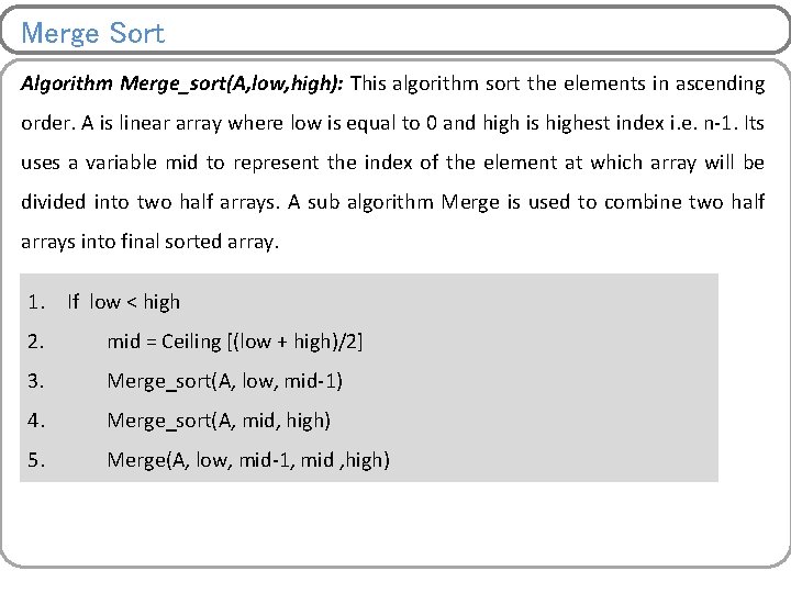
Merge Sort Algorithm Merge_sort(A, low, high): This algorithm sort the elements in ascending order. A is linear array where low is equal to 0 and high is highest index i. e. n-1. Its uses a variable mid to represent the index of the element at which array will be divided into two half arrays. A sub algorithm Merge is used to combine two half arrays into final sorted array. 1. If low < high 2. mid = Ceiling [(low + high)/2] 3. Merge_sort(A, low, mid-1) 4. Merge_sort(A, mid, high) 5. Merge(A, low, mid-1, mid , high)

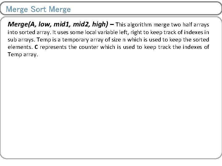
Merge Sort Merge(A, low, mid 1, mid 2, high) – This algorithm merge two half arrays into sorted array. It uses some local variable left, right to keep track of indexes in sub arrays. Temp is a temporary array of size n which is used to keep the sorted elements. C represents the counter which is used to keep track the indexes of Temp array.

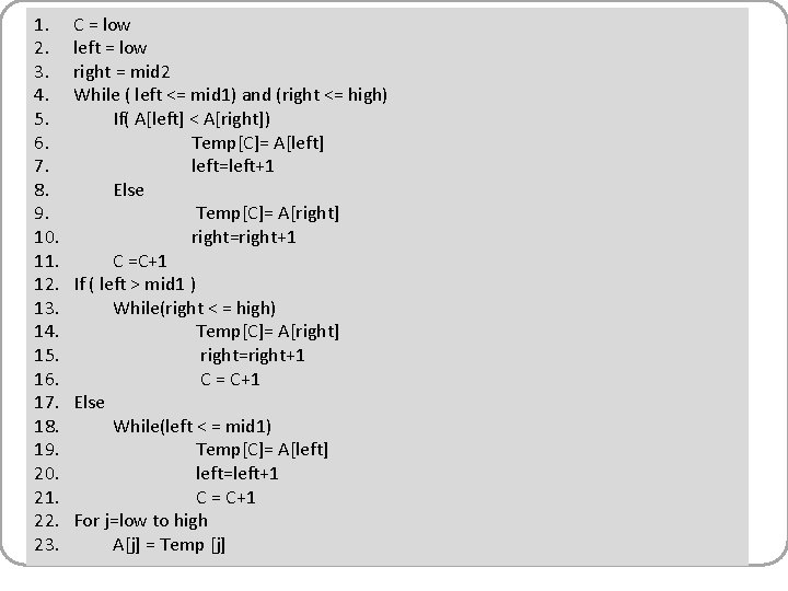
1. 2. 3. 4. 5. 6. 7. 8. 9. 10. 11. 12. 13. 14. 15. 16. 17. 18. 19. 20. 21. 22. 23. C = low left = low right = mid 2 While ( left <= mid 1) and (right <= high) If( A[left] < A[right]) Temp[C]= A[left] left=left+1 Else Temp[C]= A[right] right=right+1 C =C+1 If ( left > mid 1 ) While(right < = high) Temp[C]= A[right] right=right+1 C = C+1 Else While(left < = mid 1) Temp[C]= A[left] left=left+1 C = C+1 For j=low to high A[j] = Temp [j]

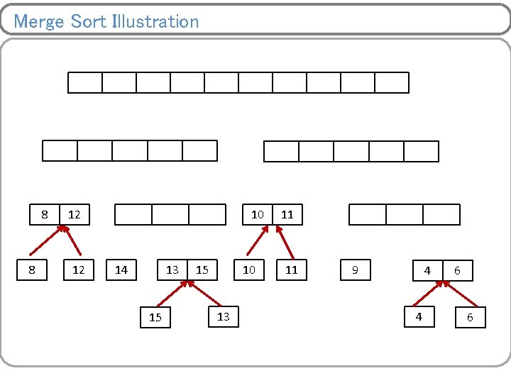
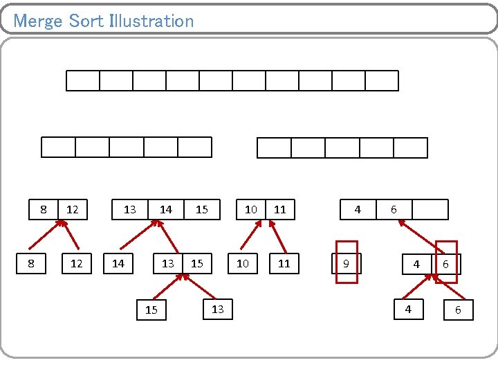
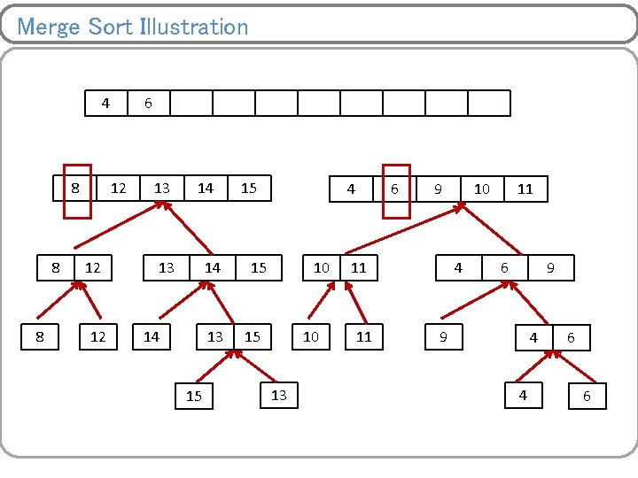
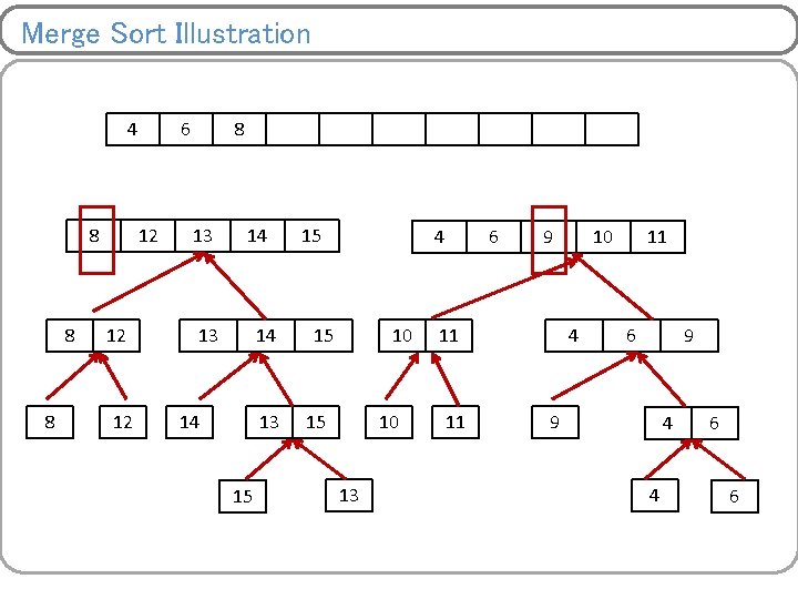
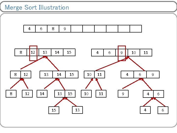
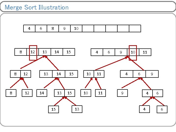
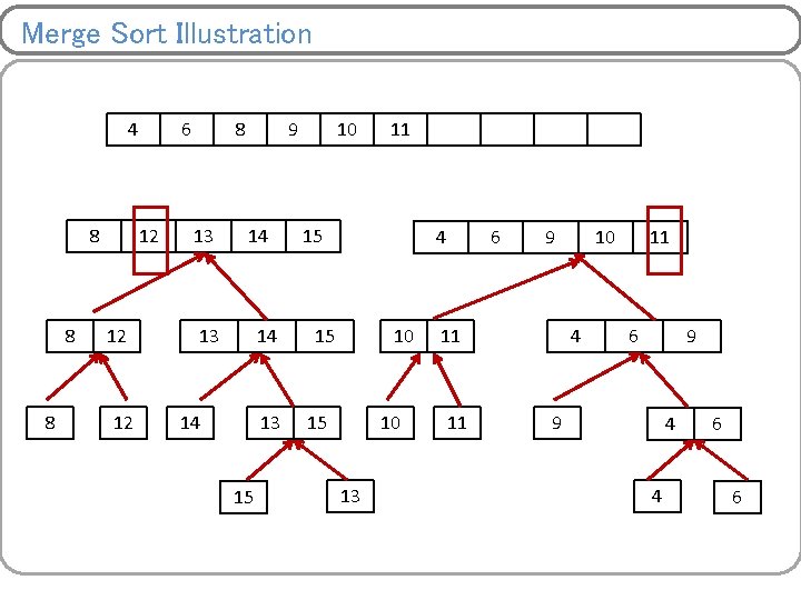
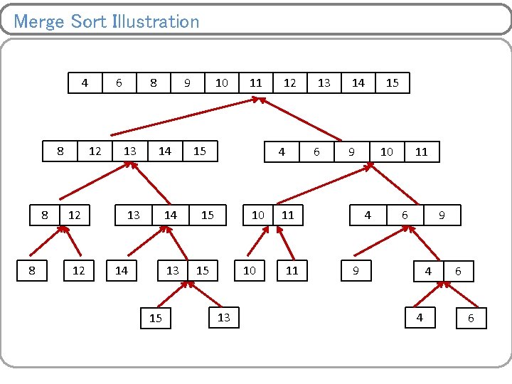
Merge Sort Illustration 8 8 12 12 14 14 15 15 13 10 13 11 10 13 9 11 4 9 11 11 6 4 9 6 4 6 9 4 4 6 6

Merge Sort Illustration 8 12 14 13 15 15 10 13 11 9 4 4 6 6

Merge Sort Illustration 8 8 12 12 10 14 13 15 15 10 13 11 11 9 4 4 6 6

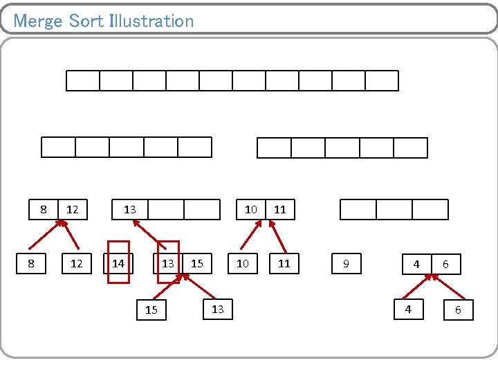
Merge Sort Illustration 8 8 12 12 13 10 14 13 15 15 10 13 11 11 9 4 4 6 6

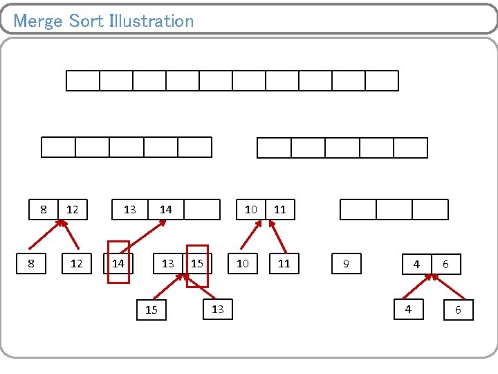
Merge Sort Illustration 8 8 12 12 13 14 14 13 15 10 13 11 11 9 4 4 6 6

Merge Sort Illustration 8 8 12 12 13 14 14 13 15 15 10 13 11 11 4 9 4 4 6 6

Merge Sort Illustration 8 8 12 12 13 14 14 13 15 15 10 13 11 11 4 6 9 4 4 6 6

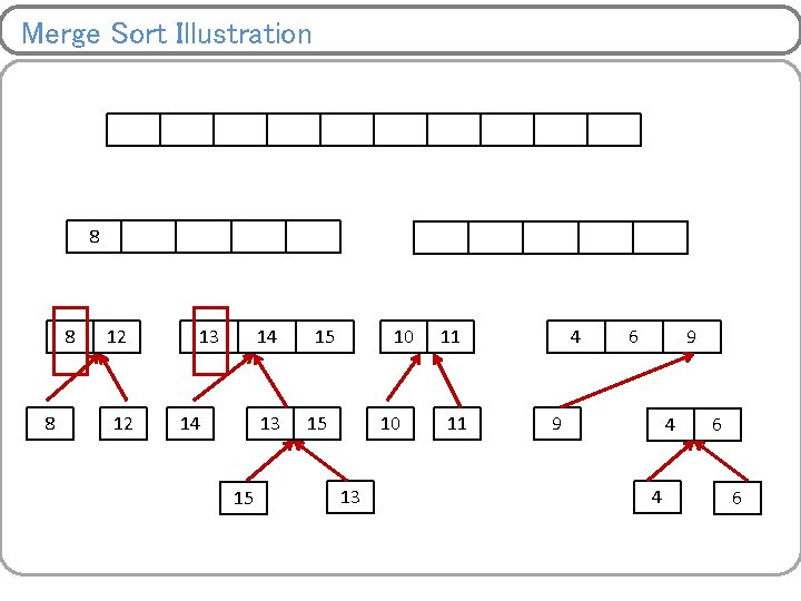
Merge Sort Illustration 8 8 8 12 12 13 14 14 13 15 15 10 13 11 11 4 6 9 9 4 4 6 6

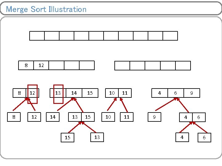
Merge Sort Illustration 8 8 8 12 12 12 13 14 14 13 15 15 10 13 11 11 4 6 9 9 4 4 6 6

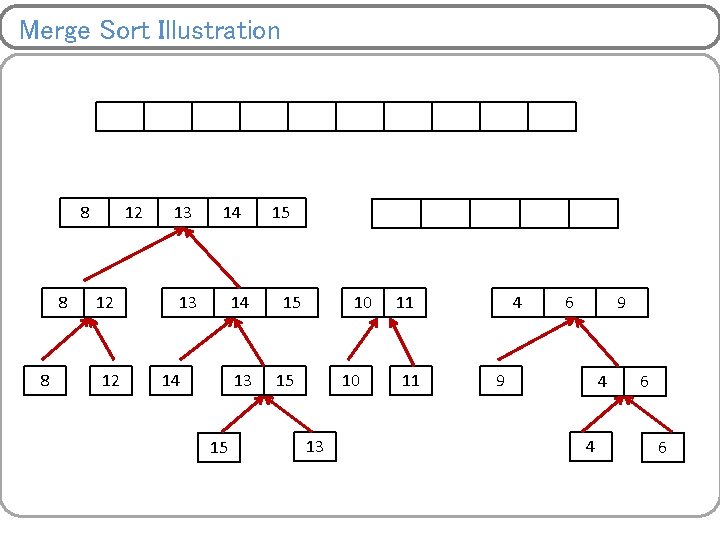
Merge Sort Illustration 8 8 8 12 12 12 13 14 14 13 15 15 15 10 13 11 11 4 6 9 9 4 4 6 6

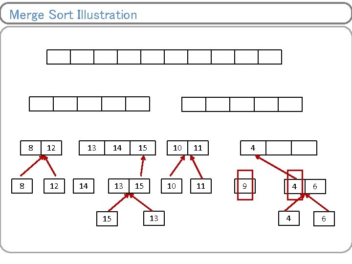
Merge Sort Illustration 8 8 8 12 12 12 13 14 14 13 15 15 4 15 10 13 11 11 4 6 9 9 4 4 6 6

Merge Sort Illustration 8 8 8 12 12 12 13 14 14 13 15 15 4 15 10 13 6 11 11 4 6 9 9 4 4 6 6

Merge Sort Illustration 8 8 8 12 12 12 13 14 14 13 15 15 4 15 10 13 6 9 11 11 4 6 9 9 4 4 6 6

Merge Sort Illustration 4 8 8 8 12 12 12 13 14 14 13 15 15 4 15 10 13 6 9 11 11 10 4 11 6 9 9 4 4 6 6

Merge Sort Illustration 4 8 8 8 6 12 12 12 13 14 14 13 15 15 4 15 10 13 6 9 11 11 10 4 11 6 9 9 4 4 6 6

Merge Sort Illustration 4 8 8 8 6 12 12 12 8 13 14 14 13 15 15 4 15 10 13 6 9 11 11 10 4 11 6 9 9 4 4 6 6

Merge Sort Illustration 4 8 8 8 6 12 12 12 8 13 9 14 13 14 14 13 15 15 4 15 10 13 6 9 11 11 10 4 11 6 9 9 4 4 6 6

Merge Sort Illustration 4 8 8 8 6 12 12 12 8 13 9 14 13 14 14 13 15 10 15 4 15 10 13 6 9 11 11 10 4 11 6 9 9 4 4 6 6

Merge Sort Illustration 4 8 8 8 6 12 12 12 8 13 9 14 13 14 14 13 15 10 11 15 4 15 10 13 6 9 11 11 10 4 11 6 9 9 4 4 6 6

Merge Sort Illustration 4 8 8 8 6 12 12 12 8 13 9 14 13 14 14 13 15 10 11 15 12 4 15 10 13 13 6 14 9 11 11 15 10 4 11 6 9 9 4 4 6 6

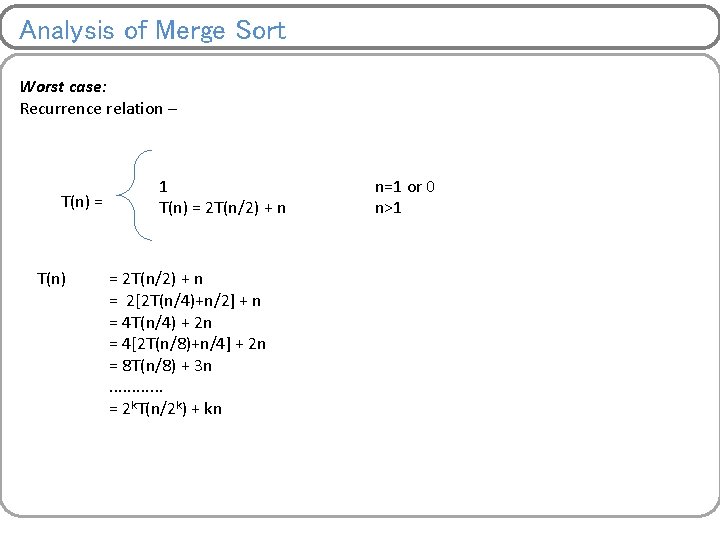
Analysis of Merge Sort Worst case: Recurrence relation – T(n) = T(n) 1 T(n) = 2 T(n/2) + n = 2[2 T(n/4)+n/2] + n = 4 T(n/4) + 2 n = 4[2 T(n/8)+n/4] + 2 n = 8 T(n/8) + 3 n. . . = 2 k. T(n/2 k) + kn n=1 or 0 n>1

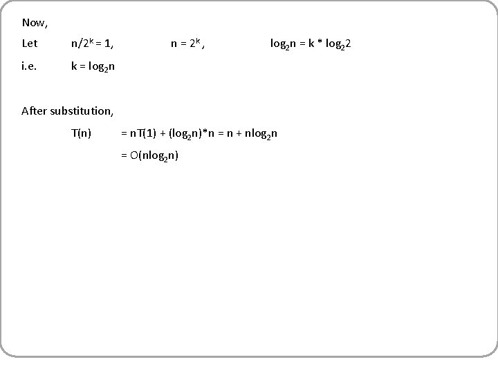
Now, Let n/2 k = 1, i. e. k = log 2 n n = 2 k , log 2 n = k * log 22 After substitution, T(n) = n. T(1) + (log 2 n)*n = n + nlog 2 n = O(nlog 2 n)

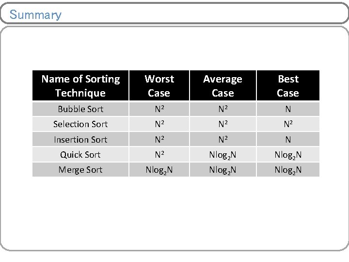
Summary Name of Sorting Technique Worst Case Average Case Best Case Bubble Sort N 2 N Selection Sort N 2 N 2 Insertion Sort N 2 N Quick Sort N 2 Nlog 2 N Merge Sort Nlog 2 N

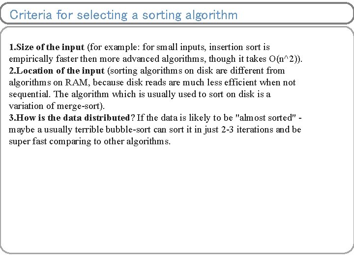
Criteria for selecting a sorting algorithm 1. Size of the input (for example: for small inputs, insertion sort is empirically faster then more advanced algorithms, though it takes O(n^2)). 2. Location of the input (sorting algorithms on disk are different from algorithms on RAM, because disk reads are much less efficient when not sequential. The algorithm which is usually used to sort on disk is a variation of merge-sort). 3. How is the data distributed? If the data is likely to be "almost sorted" maybe a usually terrible bubble-sort can sort it in just 2 -3 iterations and be super fast comparing to other algorithms.

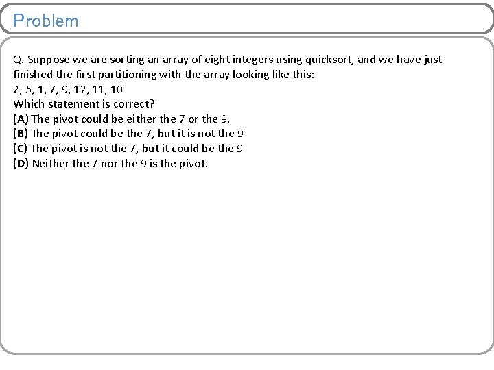
Problem Q. Suppose we are sorting an array of eight integers using quicksort, and we have just finished the first partitioning with the array looking like this: 2, 5, 1, 7, 9, 12, 11, 10 Which statement is correct? (A) The pivot could be either the 7 or the 9. (B) The pivot could be the 7, but it is not the 9 (C) The pivot is not the 7, but it could be the 9 (D) Neither the 7 nor the 9 is the pivot.