screen Lecturers desk Row A 13 8 Row

screen Lecturer’s desk Row A 13 8 Row A 7 16 15 14 20 19 18 17 16 15 Row B 21 20 19 18 17 16 Row C 22 21 20 19 18 17 Row D 23 22 21 20 19 18 Row E 17 16 15 14 13 12 11 10 9 8 7 23 22 21 20 19 18 Row F 17 16 15 14 13 12 11 10 9 8 7 24 23 22 21 20 19 Row G 18 22 21 20 19 18 17 Row H 16 14 16 24 23 22 Row J 21 20 19 18 27 26 25 24 23 Row K 22 21 20 19 28 27 26 25 24 Row L 23 28 27 26 25 24 Row M 30 29 28 27 26 Row N 25 24 23 30 29 28 27 26 Row P 25 24 23 38 9 10 17 25 39 11 18 26 40 12 19 37 36 35 34 33 23 32 22 22 31 30 Physics- atmospheric Sciences (PAS) - Room 201 21 18 9 10 8 Row B 7 4 3 2 1 Row A 6 5 4 3 2 1 Row B 14 13 12 11 10 9 8 7 Row C 6 5 4 3 2 1 Row C 15 14 13 12 11 10 9 8 7 Row D 6 5 4 3 2 1 Row D Row E 6 5 4 3 2 1 Row E Row F 6 5 4 3 2 1 Row F Row G 6 5 4 3 2 1 Row G Row H 6 5 4 3 2 1 Row H 15 14 17 18 11 5 15 16 15 12 14 13 13 12 16 12 11 10 11 table 14 19 20 21 17 13 6 9 10 8 7 9 8 7 table 13 9 8 7 6 5 1 Row J 15 14 13 12 11 10 9 8 7 6 5 4 3 2 1 Row K 17 16 15 14 13 12 11 10 9 8 7 6 5 4 3 2 1 Row L 14 13 12 11 10 9 8 7 6 5 4 3 2 1 Row M 20 19 18 17 16 15 22 21 20 19 18 17 16 15 14 13 12 11 10 9 8 7 6 5 4 3 2 1 Row N 22 21 20 19 18 17 16 15 14 13 12 11 10 9 8 7 6 5 4 3 2 1 Row P 5 4 3 2 1 Row Q 29 28 27 26 25 24 23 22 21 - 15 14 13 12 11 10 9 8 7 6

MGMT 276: Statistical Inference in Management Fall 2015

Schedule of readings Before our next exam (November 10 th) Open. Stax Chapters 1 – 10 and Chapter 13 Plous (2, 3, & 4) Chapter 2: Cognitive Dissonance Chapter 3: Memory and Hindsight Bias Chapter 4: Context Dependence

Homework On class website: Please print and complete homeworksheet #13 Hypothesis Testing using two-sample t-tests Due: Tuesday November 3 rd

By the end of lecture today 10/29/15 Logic of hypothesis testing Hypothesis testing with z-score and t-scores (one-sample) Hypothesis testing with t-scores (two independent samples) Constructing brief, complete summary statements

Homework Review mean + z σ = 30 ± (1. 96)(2) mean + z σ = 30 ± (2. 58)(2) 26. 08 < 24. 84 < µ < 33. 92 µ < 35. 16 95 % 99 %

Melvin Mark Difference not due sample size because both samples same size Difference not due population variability because same population Yes! Difference is due to sloppiness and random error in Melvin’s sample Melvin

z- score : because we know the population standard deviation Ho: µ = 5 Bags of potatoes from that plant are not different from other plants Ha: µ ≠ 5 Bags of potatoes from that plant are different from other plants Two tailed test 1. 96 (α =. 05) 1 1 = 4 =. 25 16 √ 6 – 5 = 4. 0. 25 4. 0 -1. 96 1. 9

Because the observed z (4. 0 ) is bigger than critical z (1. 96) Yes Yes . 05 These three will always match Probability of Type I error is always equal to alpha 1. 64 No Because observed z (4. 0) is still bigger than critical z (1. 64) 2. 58 No Because observed z (4. 0) is still bigger than critical z(2. 58) there is a difference there is no difference 2. 58 1. 96 there is not there is

-2. 13 2. 1 3 t- score : because we don’t know the population standard deviation Two tailed test (α =. 05) n – 1 =16 – 1 = 15 Critical t(15) = 2. 131 2. 667 89 - 85 6 √ 16

Because the observed z (2. 67) is bigger than critical z (2. 13) Yes Yes . 05 These three will always match Probability of Type I error is always equal to alpha 1. 753 No Because observed t (2. 67) is still bigger than critical t (1. 753) 2. 947 Yes Because observed t (2. 67) is not bigger than critical t(2. 947) No No No These three will always match consultant did improve morale consultant did not improve morale 2. 947 2. 13 1 she did not she did

Start summary with two means (based on DV) for two levels of the IV Finish with statistical summary z = 4. 0; p < 0. 05 Describe type of test (z-test versus t-test) with brief overview of results Or if it *were not* significant: z = 1. 2 ; n. s. = “not significant” p<0. 05 = “significant” The average weight of bags of potatoes from this particular plant Value of observedis 5 pounds. is 6 pounds, while the average weight for population statistic A z-test was completed and this difference was found to be statistically significant. We should fix the plant. (z = 4. 0; p<0. 05)

Start summary with two means (based on DV) for two levels of the IV Finish with statistical summary t(15) = 2. 67; p < 0. 05 Describe type of test (z-test versus t-test) with brief overview of results Or if it *were not* significant: t(15) = 1. 07; n. s. = “not significant” p<0. 05 = “significant” The average job-satisfaction score was 89 for Value the employees who went of observed On the retreat, while the average score for population is 85. A t-test statistic df was completed and this difference was found to be statistically significant. We should hire the consultant. (t(15) = 2. 67; p<0. 05)

Five steps to hypothesis testing Step 1: Identify the research problem (hypothesis) Describe the null and alternative hypotheses Step 2: Decision rule • • Alpha level? (α =. 05 or. 01)? One or two tailed test? Balance between Type I versus Type II error Critical statistic (e. g. z or t or F or r) value? Step 3: Calculations Step 4: Make decision whether or not to reject null hypothesis If observed z (or t) is bigger then critical z (or t) then reject null Step 5: Conclusion - tie findings back in to research problem

Is this a single sample or two sample test? Is it a z or a t test or an ANOVA? Hypothesis testing Is it a one-tail test or a two tail test? Step 1: Identify the research problem Did the sheriff keep her promise to change response times from the previous average of 30 minutes? Step 2: Describe the null and alternative hypotheses Ho: The response times are not changed H 1: The response times did change As the new chief of police, I am going to change response times for traffic accidents. Before I started the average response time was 30 minutes

Hypothesis testing Gather the data: We measured the time for police to respond to 10 accidents Two-tailed • • test One or two tailed test? n= 10 What is our sample size What is size of our degrees of freedom? alpha = What is our alpha What is our critical t value? 0. 05 n = 10 (df = 9) Alpha =. 05 Decision rule: critical t = 2. 62 df = 9

Hypothesis testing Gather the data: We measured the time for police to respond to 10 accidents • One or two tailed test? • What is our sample size • What is size of our degrees of freedom? • What is our alpha • What is our critical t value? • Decision rule: critical t = 2. 262 Two-tailed test Alpha of 0. 05 Critical t (9) = 2. 262

Step 3: Calculations: • Average time for response before 30 minutes • Average time for response after 24 minutes • Observed t = - 2. 71 Step 4: Make decision whether or not to reject null hypothesis Observed t = - 2. 71 Critical t = 2. 262 -2. 71 is farther out on the curve than 2. 262 so, we do not reject the null hypothesis Step 5: Conclusion: There appears to be a significant difference between the sheriff’s times and 30 minutes

Hypothesis testing: Did the sheriff keep her promise to reduce response times to less than 30 minutes? Start summary with two means (based on DV) for two levels of the IV Describe type of test (t-test versus anova) with brief overview of results notice we are comparing a sample mean with a population mean: single sample t-test Finish with statistical summary t(9) = -5. 71; p < 0. 05 Or if it had been different results that *were not* significant: t(9) = -1. 71; ns The mean response time for following the sheriff’s new plan was 24 minutes, while the mean response time prior to the new plan was 30 minutes. A t-test was completed and there appears to be a significant difference in the response time following the implementation of the new plan t(9) = -2. 71; p < 0. 05 Type of test with degrees of freedom Value of observed statistic n. s. = “not significant” p<0. 05 = “significant”

. . A note on z scores, and t score: • Numerator is always distance between means (how far away the distributions are) • Denominator is always measure of variability (how wide or much overlap there is between distributions) Difference between means Variability of curve(s)

Five steps to hypothesis testing Step 1: Identify the research problem (hypothesis) How is a single sample t-test different Describe the null and alternative hypotheses than two sample t-test? How. Step is a single samplerule t-test most 2: Decision similar to the two sample t-test? • Alpha level? (α =. 05 or. 01)? • Critical statistic (e. g. z or t) value? Step 3: Calculations Step 4: Make decision whether or not to reject null hypothesis If observed z (or t) is bigger then critical z (or t) then Single sample standard has one “n” reject null deviation average while two versus samples will have for Step 5: Conclusion - tie findings backstandard in to problem an “n”research fordeviation each sample two samples

Independent samples t-test Are the two means significantly different from each other, or is the difference just due to chance? Donald is a consultant and leads training sessions. As part of his training sessions, he provides the students with breakfast. He has noticed that when he provides a full breakfast people seem to learn better than when he provides just a small meal (donuts and muffins). So, he put his hunch to the test. He had two classes, both with three people enrolled. The one group was given a big meal and the other group was given only a small meal. He then compared their test performance at the end of the day. Please test with an alpha =. 05 Small meal Big Meal 19 22 23 25 21 25 Mean= 21 Mean= 24 x 1 – x 2 t= variability 24 – 21 t = variability Got to figure this part out: We want to average from 2 samples - Call it “pooled”

Hypothesis testing Step 1: Identify the research problem Did the size of the meal affect the learning / test scores? Step 2: Describe the null and alternative hypotheses Ho: The size of the meal has no effect on test scores H 1: The size of the meal does have an effect on test scores Step 3: Decision rule α =. 05 One tail or two tail test?

Hypothesis testing Step 3: Decision rule α =. 05 n 1 = 3; n 2 = 3 Degrees of freedom total (df total) = (n 1 - 1) + (n 2 – 1) = (3 - 1) + (3 – 1) = 4 Degrees of freedom total (df total) = (n total - 2) two tailed test Critical t(4) = 2. 776 Notice: Two different ways to think about it

two tail test α=. 05 (df) = 4 Critical t(4) = 2. 776

Mean= 21 Mean= 24 Big Meal Deviation Squared Big Meal From mean deviation -2 22 4 1 25 1 Σ=6 1 1 2 S 2 2 pooled S 2 pooled = = 6 2 8 2 Small meal 19 23 21 Small Meal Deviation From mean -2 2 0 Σ=8 = 1. 732 = 2. 0 Notice: s 2 = 3. 0 Notice: s 2 = 4. 0 (n 1 – 1) s 12 + (n 2 – 1) s 22 n 1 + n 2 - 2 (3 – 1) (1. 732) 2 + (3 – 1) (2)2 31 + 32 - 2 Squared Deviation 4 4 0 = 3. 5 Notice: Simple Average = 3. 5

Mean= 21 Mean= 24 Big Meal Deviation Squared Participant Big Meal From mean deviation -2 22 1 4 1 25 2 1 1 25 3 1 Σ=6 Small meal 19 23 21 Small Meal Deviation From mean -2 2 0 Squared Deviation 4 4 0 Σ=8 S 2 p = 3. 5 24 - 21 3. 5 3 = 24 – 21 1. 5275 = 1. 964 Observed t

Hypothesis testing Step 5: Make decision whether or not to reject null hypothesis Observed t = 1. 964 Critical t = 2. 776 1. 964 is not farther out on the curve than 2. 776 so, we do not reject the null hypothesis t(4) = 1. 964; n. s. Step 6: Conclusion: There appears to be no difference in test scores between the two groups

Mean of small meal was 21 Mean of big meal was 24 How to report the findings for a t-test One paragraph summary of this study. Describe the IV & DV. Present the two means, which type of test was conducted, and the statistical results. Finish with statistical Observed t = 1. 964 Start summary with two summary means (based on DV) t(4) = 1. 96; ns df = 4 for two levels of the IV Describe type of test (t-test versus anova) with brief overview of results Or if it *were* significant: t(9) = 3. 93; p < 0. 05 We compared test scores for large and small meals. The mean test scores for the big meal was 24, and was 21 for the small meal. A t-test was calculated and there appears to be no significant difference in test scores between the two types of meals t(4) = 1. 964; n. s. Type of test with degrees of freedom Value of observed statistic n. s. = “not significant” p<0. 05 = “significant”

Mean= 21 Mean= 24 Participant Big Meal 22 1 25 2 25 3 Small meal 19 23 21 Figuring out the two means using Excel

Mean= 21 Mean= 24 Participant Big Meal 22 1 25 2 25 3 Small meal 19 23 21 Figuring out the two means

Mean= 21 Mean= 24 Participant Big Meal 22 1 25 2 25 3 Figuring out the two means Small meal 19 23 21 Mean= 24

Mean= 21 Complete a t-test Mean= 24 Participant Big Meal 22 1 25 2 25 3 May want to remove means so don’t include in the t-test Small meal 19 23 21

Mean= 21 Complete a t-test Mean= 24 Participant Big Meal 22 1 25 2 25 3 Small meal 19 23 21 If checked you’ll want to to If checked, include the labels in your variable range

Finding Means

Finding degrees of freedom

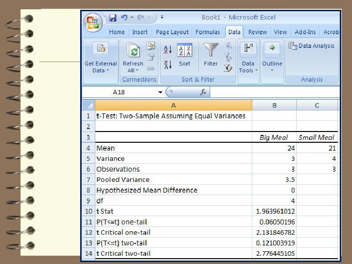
Finding Observed t

Finding Critical t

Finding p value (Is it less than. 05? )

Mean of small meal was 21 Mean of big meal was 24 How to report the findings for a t-test One paragraph summary of this study. Describe the IV & DV. Present the two means, which type of test was conducted, and the statistical results. Finish with statistical Observed t = 1. 964 Start summary with two summary means (based on DV) t(4) = 1. 96; ns df = 4 for two levels of the IV Describe type of test (t-test versus anova) with brief overview of results Or if it *were* significant: t(9) = 3. 93; p < 0. 05 We compared test scores for large and small meals. The mean test scores for the big meal was 24, and was 21 for the small meal. A t-test was calculated and there appears to be no significant difference in test scores between the two types of meals t(4) = 1. 964; n. s. Type of test with degrees of freedom Value of observed statistic n. s. = “not significant” p<0. 05 = “significant”