Screen Lecturers desk Row A Row B Row

Screen Lecturer’s desk Row A Row B Row A 15 14 12 11 10 13 20 Row B 19 24 23 22 21 Row C 20 19 28 27 26 25 24 23 Row D 22 21 20 19 30 29 28 27 26 25 24 23 Row E 23 22 21 20 19 35 34 33 32 31 30 29 28 27 26 Row F 25 35 34 33 32 31 30 29 28 27 26 Row G 37 36 35 34 33 32 31 30 29 28 41 40 39 38 37 36 35 34 33 32 31 30 Row C Row D Row E Row F Row G Row H Row L 33 31 29 25 23 22 21 21 8 7 6 5 3 4 Row A 2 1 3 2 Row B 9 8 7 6 5 4 12 11 10 9 8 7 6 5 4 3 2 1 24 23 22 21 20 19 18 17 16 15 14 13 12 11 10 9 8 7 6 5 4 3 2 1 Row F 25 24 23 22 21 20 19 18 17 16 15 14 13 12 11 10 9 8 7 6 5 4 3 2 1 Row G Row H 27 26 25 24 23 22 21 20 19 18 17 16 15 14 13 12 29 Row J 28 27 26 25 24 23 22 21 20 19 18 17 16 15 14 13 12 11 10 9 8 7 6 5 4 3 2 1 Row J 29 Row K 28 27 26 25 24 23 22 21 20 19 18 17 16 15 14 13 12 11 10 9 8 7 6 5 4 3 2 1 Row K 25 Row L 24 23 22 21 20 19 18 17 16 15 14 13 12 11 10 9 20 19 Row M 18 4 3 Row N 15 14 13 12 11 10 9 8 7 6 5 4 3 2 1 Row P 15 14 13 12 11 10 9 8 7 6 5 4 3 2 1 4 3 32 31 30 29 28 27 26 Row M 9 18 17 18 16 17 15 16 18 14 15 17 18 13 14 13 16 17 12 11 10 15 16 14 15 13 12 11 10 14 17 16 15 14 13 12 11 10 9 13 8 7 6 5 1 1 Row C Row D Row E 11 10 9 8 7 6 5 4 3 2 2 1 1 1 Row L Row M table 14 13 12 11 10 9 8 7 6 Projection Booth Harvill 150 renumbered 5 2 1 Left handed desk Row H

Introduction to Statistics for the Social Sciences SBS 200 - Lecture Section 001, Fall 2018 Room 150 Harvill Building 10: 00 - 10: 50 Mondays, Wednesdays & Fridays. 11/19/18

A note on doodling

Extra Credit Assignment Due November 19 n i d n a h e s a Ple t i d e r C a r t Ex t n e m n g i s s A
 Open. Stax")
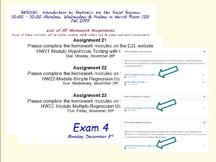
Schedule of readings Before our fourth and final exam (December 3 rd) Open. Stax Chapters 1 – 13 (Chapter 12 is emphasized) Plous Chapter 17: Social Influences Chapter 18: Group Judgments and Decisions

Over next couple of lectures 11/19/18 Logic of hypothesis testing with Correlations Interpreting the Correlations and scatterplots Simple and Multiple Regression Using correlation for predictions r versus r 2 Regression uses the predictor variable (independent) to make predictions about the predicted variable (dependent) Coefficient of correlation is name for “r” Coefficient of determination is name for “r 2” (remember it is always positive – no direction info) Standard error of the estimate is our measure of the variability of the dots around the regression line (average deviation of each data point from the regression line – like standard deviation) Coefficient of regression will “b” for each variable (like slope)

s b a k L e Nois we th

ay d s dne e W ay! n o lid s o s a H cl y o N Happ

Scatterplot displays relationships between two continuous variables Correlation: Measure of how two variables co-occur and also can be used for prediction Range between -1 and +1 The closer to zero the weaker the relationship and the worse the prediction Positive or negative

Positive correlation: as values on one variable go up, so do values for the other variable Negative correlation: as values on one variable go up, the values for the other variable go down Positive Correlation Brushing teeth by number cavities Height of Daughters Perfect Correlation Height (inches) by height (centimeters) Height in inches Brushing Teeth Height of Mothers by height of Daughters Negative Correlation Number Cavities Height in Centimeters

Correlation - How do numerical values change? r = +0. 97 r = -0. 91 r = -0. 48 r = 0. 61 Revisit this slide

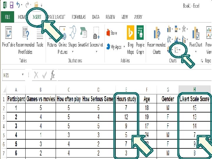
Predicting One positive correlation “Passion for Gaming” Score Time Studying 15 12 9 6 3 0 3 6 9 12 15 20 Final results might look like this
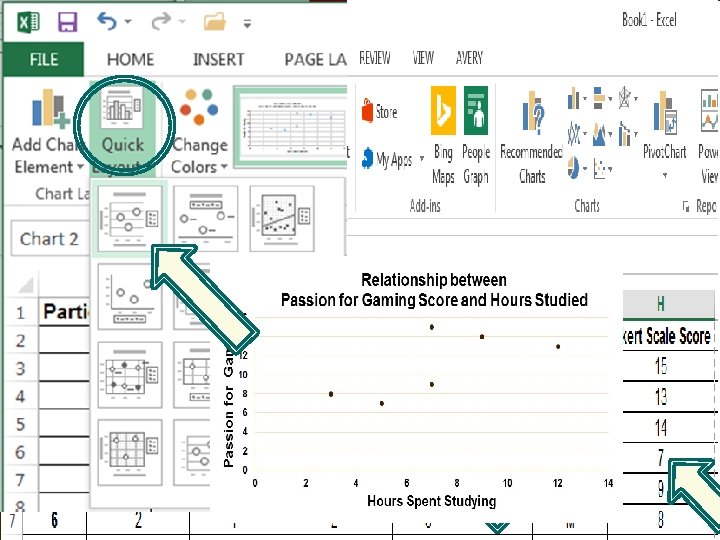

Regression: Predicting level of passion for gaming r = 0. 67 b =. 7372 (slope) a = 5. 72 (intercept) Step 1: Draw prediction line Right click on dots Draw a regression line and regression equation

Regression: Predicting level of passion for gaming Step 1: Draw prediction line Draw a regression line and regression equation r = 0. 67 b =. 7372 (slope) a = 5. 72 (intercept)

Regression: Predicting level of passion for gaming Step 1: Draw prediction line Draw a regression line and regression equation r = 0. 67 b =. 7372 (slope) a = 5. 72 (intercept)

Regression: Predicting level of passion for gaming Step 1: Draw prediction line Draw a regression line and regression equation r = 0. 67 b =. 7372 (slope) a = 5. 72 (intercept)
 Describe relationship r")
Regression: Predicting level of passion for gaming Regression line (and equation) Describe relationship r =. 67 Correlation: This is a strong positive correlation. Passion tends to increase as number of hours increase Predict using regression line (and regression equation) b =. 7372 (slope) Dependent Variable Independent Variable Intercept: suggests that we can assume each person starts with Slope: for each additional hour spent studying, passion increase by. 7372 points a = 5. 72 (intercept)

Predicting One positive correlation “Number Systems Sold” Number of Sales Calls 80 60 40 20 0 0 3 6 9 12 15 20 Final results might look like this
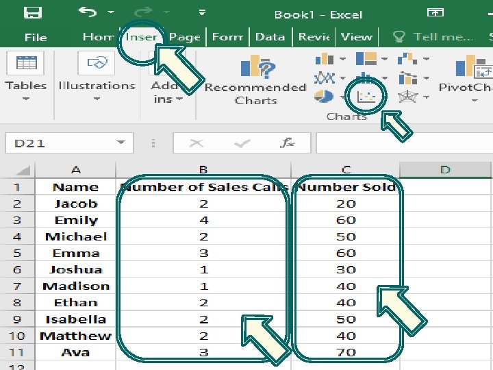
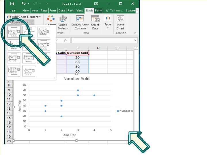

Regression: Predicting sales from sales calls Step 1: Draw prediction line Right click on dots Draw a regression line and regression equation

Regression: Predicting sales from sales calls Step 1: Draw prediction line r = 0. 7068 b = 11. 579(slope) a = 20. 526 (intercept) Choose Display Equation and Display R-squared Draw a regression line and regression equation

Regression: Predicting sales from sales calls Step 1: Draw prediction line Draw a regression line and regression equation r = 0. 7068 b = 11. 579(slope) a = 20. 526 (intercept)
 Describe relationship r =")
Regression: Predicting sales from sales calls Regression line (and equation) Describe relationship r = 0. 7068 Correlation: This is a strong positive correlation. Sales tend to increase as number of sales calls increase Predict using regression line (and regression equation) b = 11. 579(slope) Dependent Variable Independent Variable Intercept: suggests that we can assume each person starts with Slope: for each additional sales call, sales increase by 11. 579. a = 20. 526 (intercept)

s, mo t e o d l erp me i t t t a l Rea lete sc imple s mp d o n c a el c o s x t n E o How orrelati s using c sion s e r reg http: //courses. eller. arizona. edu/mgmt/delaney/Donalds. Used. Cars. Data. xlsx
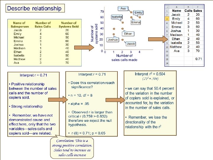

Summary Intercept: suggests that we can assume each salesperson will sell at least 20. 526 systems Slope: as sales calls increase by one, 11. 579 more systems should be sold w R e i v e

- Slides: 31