Screen Lecturers desk Row A Row B Row

Screen Lecturer’s desk Row A Row B Row A 15 14 12 11 10 13 20 Row B 19 24 23 22 21 Row C 20 19 28 27 26 25 24 23 Row D 22 21 20 19 30 29 28 27 26 25 24 23 Row E 23 22 21 20 19 35 34 33 32 31 30 29 28 27 26 Row F 25 35 34 33 32 31 30 29 28 27 26 Row G 37 36 35 34 33 32 31 30 29 28 41 40 39 38 37 36 35 34 33 32 31 30 Row C Row D Row E Row F Row G Row H Row L 33 31 29 25 23 22 21 21 8 7 6 5 3 4 Row A 2 1 3 2 Row B 9 8 7 6 5 4 12 11 10 9 8 7 6 5 4 3 2 1 24 23 22 21 20 19 18 17 16 15 14 13 12 11 10 9 8 7 6 5 4 3 2 1 Row F 25 24 23 22 21 20 19 18 17 16 15 14 13 12 11 10 9 8 7 6 5 4 3 2 1 Row G Row H 27 26 25 24 23 22 21 20 19 18 17 16 15 14 13 12 29 Row J 28 27 26 25 24 23 22 21 20 19 18 17 16 15 14 13 12 11 10 9 8 7 6 5 4 3 2 1 Row J 29 Row K 28 27 26 25 24 23 22 21 20 19 18 17 16 15 14 13 12 11 10 9 8 7 6 5 4 3 2 1 Row K 25 Row L 24 23 22 21 20 19 18 17 16 15 14 13 12 11 10 9 20 19 Row M 18 4 3 Row N 15 14 13 12 11 10 9 8 7 6 5 4 3 2 1 Row P 15 14 13 12 11 10 9 8 7 6 5 4 3 2 1 4 3 32 31 30 29 28 27 26 Row M 9 18 17 18 16 17 15 16 18 14 15 17 18 13 14 13 16 17 12 11 10 15 16 14 15 13 12 11 10 14 17 16 15 14 13 12 11 10 9 13 8 7 6 5 table 15 14 13 12 11 10 9 8 7 6 Projection Booth 5 2 1 1 1 Row C Row D Row E 11 10 9 8 7 6 5 4 3 2 2 1 1 1 Row L Row M Harvill 150 renumbered Left handed desk Row H

Screen Kristina Lecturer’s desk Row A Attila Row C Row B Row A 15 14 12 11 10 13 20 Row B 19 24 23 22 21 Row C 20 19 28 27 26 25 24 23 Row D 22 21 20 19 30 29 28 27 26 25 24 23 Row E 23 22 21 20 19 35 34 33 32 31 30 29 28 27 26 Row F 25 35 34 33 32 31 30 29 28 27 26 Row G 37 36 35 34 33 32 31 30 29 28 41 40 39 38 37 36 35 34 33 32 31 30 25 Row D Row E Row F Row G Row H Row L 33 31 29 23 22 21 Ha nn a h 21 8 7 6 5 Row A 2 1 3 2 Row B 8 7 6 5 4 12 11 10 9 8 7 6 5 4 3 2 1 24 23 22 21 20 19 18 17 16 15 14 13 12 11 10 9 8 7 6 5 4 3 2 25 24 23 22 21 20 19 18 17 16 15 14 13 12 11 10 9 8 7 6 5 4 3 2 Row H 27 26 25 24 23 22 21 20 19 18 17 16 15 14 13 12 29 Row J 28 27 26 25 24 23 22 21 20 19 18 17 16 15 14 13 12 11 10 9 8 7 6 5 4 3 2 1 Row J 29 Row K 28 27 26 25 24 23 22 21 20 19 18 17 16 15 14 13 12 11 10 9 8 7 6 5 4 3 2 1 Row K 25 Row L 24 23 22 21 20 19 18 17 16 15 14 13 12 11 10 9 20 19 Row M 18 4 3 Row N 15 14 13 12 11 10 9 8 7 6 5 4 3 2 1 Row P 15 14 13 12 11 10 9 8 7 6 5 4 3 2 1 4 3 18 17 18 16 17 15 16 18 14 15 17 18 13 14 13 16 17 12 11 10 15 16 14 15 13 12 11 10 14 17 16 15 14 13 12 11 10 9 13 8 7 6 5 table 14 13 12 11 10 9 8 7 6 Projection Booth Harvill 150 renumbered 3 4 9 32 31 30 29 28 27 26 Row M 9 5 2 1 1 Row C Row D le l e h. Row F Row E M ic 1 1 Row G 11 10 9 8 7 6 5 4 3 2 2 1 1 1 Row L Row M e Sez n 1 Left handed desk Row H

Introduction to Statistics for the Social Sciences SBS 200 - Lecture Section 001, Spring 2018 Room 150 Harvill Building 9: 00 - 9: 50 Mondays, Wednesdays & Fridays. 1/31/18 http: //www. youtube. com/watch? v=o. SQJP 40 Pc. GI

Everyone will want to be enrolled in one of the lab sessions Labs c ontinu e this w eek

n o i at l e r or ow C n s i t h n t shee i nd ork a H W

In nearly every class we will use clickers to answer questions in class and participate in interactive class demonstrations e v a h u o y f i d e r Even e t s i g e r t e y n a c t o u n o y r e k c i l c r e u t a yo p i c i t r a p still
 Please read chapters 1 - 5")
Schedule of readings Before next exam (February 9) Please read chapters 1 - 5 in Open. Stax textbook Please read Appendix D, E & F online On syllabus this is referred to as online readings 1, 2 & 3 Please read Chapters 1, 5, 6 and 13 in. Plous Chapter 1: Selective Perception Chapter 5: Plasticity Chapter 6: Effects of Question Wording and Framing Chapter 13: Anchoring and Adjustment

You’ve gathered your data…what’s the best way to display it? ?

14 16 Lists of numbers 11 too hard to see 20 patterns 14 Describing Data Visually 11 16 11 8 11 14 14 8 12 14 10 9 12 15 10 13 15 11 13 16 11 14 16 17 25 21 28 16 14 12 14 17 18 17 13 17 17 18 18 18 19 20 27 19 16 8 17 25 16 19 23 20 15 20 20 20 21 21 22 23 24 25 18 24 13 17 19 9 18 24 12 25 11 25 25 27 28 29 21 16 20 17 17 24 20 22 15 11 Organizing numbers helps Graphical representation even more clear This is a dot plot 29 13 11 14 11 8 17

Describing Data Visually 8 8 9 10 11 11 12 12 13 13 13 14 14 14 15 15 16 16 16 17 17 17 18 18 18 19 19 20 20 21 21 22 23 24 24 25 25 25 27 28 29 Graphical representation even more clear This is a dot plot

Describing Data Visually 8 8 9 10 11 11 11 12 12 13 13 14 14 We’ve got to put these data into groups (“bins”) 14 14 15 15 16 16 16 17 17 17 18 18 18 19 19 20 20 21 21 22 23 24 24 25 25 25 27 28 29 Measuring the “frequency of occurrence” Then figure “frequency of occurrence” for the bins

Frequency distributions an organized list of observations and their frequency of occurrence How many kids are in your family? What is the most common family size?

Another example: How many kids in your family? Number of kids in family 1 3 1 4 2 8 2 14 14 4 2 1 4 2 2 3 1 8

How many kids are in your family? What is the most common family size? Frequency distributions Crucial guidelines for constructing frequency distributions: Number of kids in family 1 3 1 4 2 8 2 14 1. Classes should be mutually exclusive: Each observation should be represented only once (no overlap between classes) 5 and 10 appear in multiple groups Wrong 0 -5 5 - 10 10 - 15 Correct 0 -4 5 -9 10 - 14 Correct 0 - under 5 5 - under 10 10 - under 15 2. Set of classes should be exhaustive: Wrong Should include all possible data values 0 -4 (no data points should fall outside range) 8 - 11 12 - 15 Missing 5, 6 and 7 Correct 0 -3 4 -7 8 - 11 12 - 15

How many kids are in your family? What is the most common family size? Frequency distributions Crucial guidelines for constructing frequency distributions: Number of kids in family 1 3 1 4 2 8 2 14 3. All classes should have equal intervals (even if the frequency for that class is zero) Wrong 0 -1 2 - 12 14 - 15 Correct 0 -4 5 -9 10 - 14 Correct 0 - under 5 5 - under 10 10 - under 15

4. Selecting number of classes is subjective How about Generally 5 -15 will often work 6 classes? (“bins”) How about 8 classes? (“bins”) 8 8 9 10 11 11 11 12 12 13 13 14 14 14 15 15 16 16 16 17 17 17 18 18 18 19 19 20 20 21 21 22 23 24 How about 16 classes? (“bins”) 24 25 25 25 27 28 29
 numbers Remember: This is all about helping")
5. Class width should be round (easy) numbers Remember: This is all about helping readers understand quickly and clearly. Lower boundary can be multiple of interval size Round numbers: 5, 10, 15, 20 etc or 6. Try to avoid open ended 3, 6, 9, 12 classes For example etc • 10 and above • Greater than 100 • Less than 50 Clear & Easy 8 - 11 12 - 15 16 - 19 20 - 23 24 - 27 28 - 31 8 8 9 10 11 11 11 12 12 13 13 14 14 14 15 15 16 16 16 17 17 17 18 18 18 19 19 20 20 21 21 22 23 24 24 25 25 25 27 28 29

Scores on an exam Step 6: Complete the Frequency Table Scores on an exam Relative Cumulative Score Frequency 95 - 99 2. 0715 28 1. 0000 90 - 94 3. 1071 26. 9285 85 - 89 5. 1786 23. 8214 80 – 84 5. 1786 18. 6428 75 - 79 4. 1429 13. 4642 70 - 74 3. 1071 9. 3213 65 - 69 1. 0357 6. 2142 60 - 64 3. 1071 5. 1785 55 - 59 1. 0357 2. 0714 50 - 54 1. 0357 6 bins Just adding Interval of 8 up the frequency data from the smallest to largest numbers Just dividing each frequency by total number to get a ratio (like a percent) 82 75 88 93 53 84 87 Please note: 1 /28 =. 0357 3/ 28 =. 1071 4/28 =. 1429 58 64 80 72 87 73 94 84 78 69 70 60 84 76 87 Just adding 61 89 95 up the 91 75 99 relative frequency data from the smallest to. Please largestnote: numbers Also just dividing cumulative frequency by total number 1/28 =. 0357 2/28 =. 0714 5/28 =. 1786

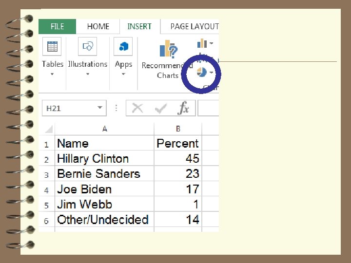
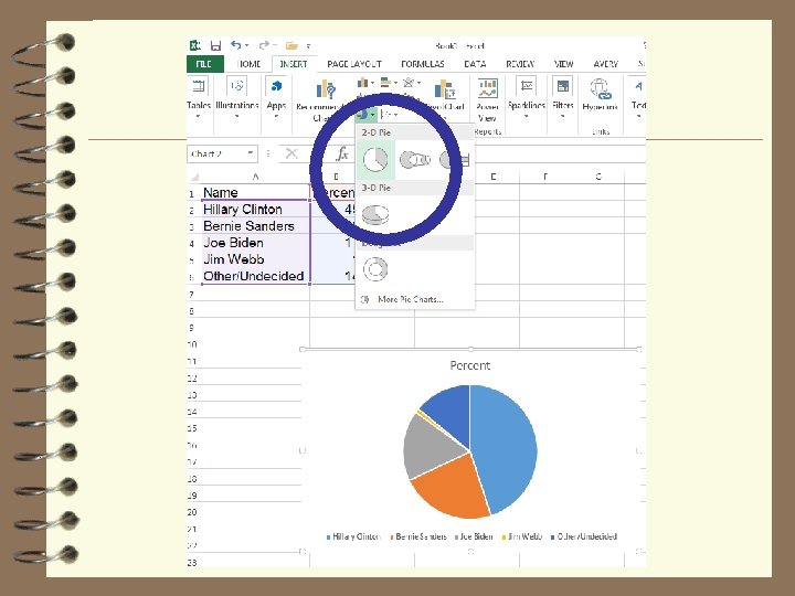
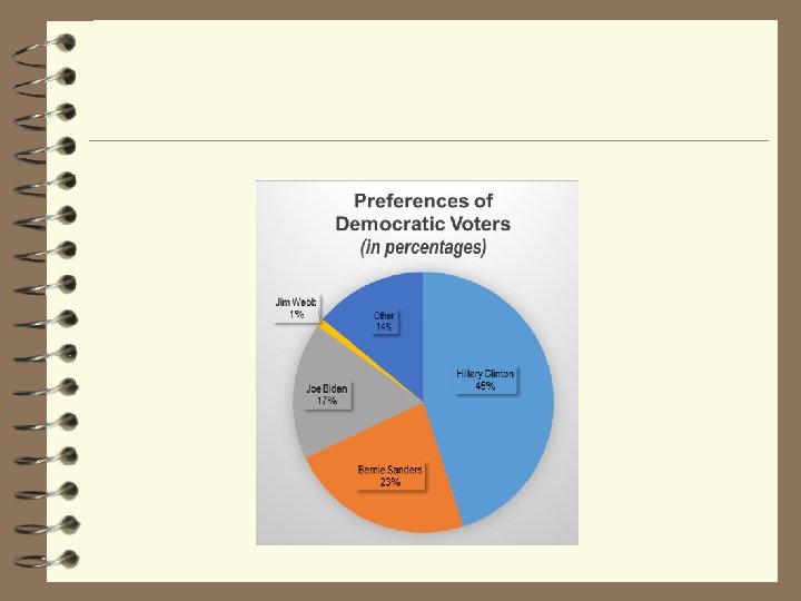
Simple Frequency Table – Qualitative Data Who is your favorite candidate Candidate Frequency Hillary Clinton 45 Bernie Sanders 23 Joe Biden 17 Jim Webb 1 Other/Undecided 14 Relative Frequency. 4500. 2300. 1700. 0100. 1400 Just divide each frequency by total number Please note: 45 /100 =. 4500 23 /100 =. 2300 17 /100 =. 1700 1 /100 =. 0100 Percent 45% 23% 17% 1% 14% Number expected to vote 9, 900, 000 5, 060, 000 3, 740, 000 220, 000 3, 080, 000 Just multiply each relative frequency by 100 Please note: . 4500 x 100 = 45%. 2300 x 100 = 23%. 1700 x 100 = 17%. 0100 x 100 = 1% We asked 100 Democrats “Who is your favorite candidate? ” If 22 million Democrats voted today how many would vote for each candidate? Just multiply each relative frequency by 22 million Please note: . 4500 x 22 m = 9, 900 k. 2300 x 22 m = 35, 060 k. 1700 x 22 m = 23, 740 k. 0100 x 22 m= 220 k Data based on Gallup poll on 8/24/11

Describing Data Visually 8 8 9 10 11 11 12 12 13 13 13 14 14 14 15 15 16 16 16 17 17 17 18 18 18 19 19 20 20 21 21 22 23 24 24 25 25 25 27 28 29 Graphical representation even more clear This is a dot plot

Scores on an exam Remember Dot Plots Step 1: List scores Step 2: List scores in order Step 3: Decide grouped 82 75 88 93 53 84 87 Step 4: Decide 10 for # bins (classes) 5 for bin width (interval size) Step 5: Generate frequency histogram 58 72 94 69 84 61 91 64 87 84 70 76 89 75 80 73 78 60 87 95 99 6 5 4 3 2 1 9 4 50 -5 55 -5 4 60 -6 4 9 65 -6 70 -7 75 9 -7 4 80 Score on exam -8 9 85 -8 4 90 -9 9 95 -9 Scores on an exam Score Frequency 95 - 99 2 90 - 94 3 85 - 89 5 80 – 84 5 75 - 79 4 70 - 74 3 65 - 69 1 60 - 64 3 55 - 59 1 50 - 54 1 53 58 60 61 64 69 70 72 73 75 75 76 78 80 82 84 84 84 87 87 87 88 89 91 93 94 95 99

Scores on an exam Remember Dot Plots Step 1: List scores Step 2: List scores in order Step 3: Decide grouped 82 75 88 93 53 84 87 Step 4: Decide 10 for # bins (classes) 5 for bin width (interval size) Step 5: Generate frequency histogram 58 72 94 69 84 61 91 64 87 84 70 76 89 75 80 73 78 60 87 95 99 6 5 4 3 2 1 9 4 50 -5 55 -5 4 60 -6 4 9 65 -6 70 -7 75 9 -7 4 80 Score on exam -8 9 85 -8 4 90 -9 9 95 -9 Scores on an exam Score Frequency 95 - 99 2 90 - 94 3 85 - 89 5 80 – 84 5 75 - 79 4 70 - 74 3 65 - 69 1 60 - 64 3 55 - 59 1 50 - 54 1 53 58 60 61 64 69 70 72 73 75 75 76 78 80 82 84 84 84 87 87 87 88 89 91 93 94 95 99

Scores on an exam Remember Dot Plots Step 1: List scores Step 2: List scores in order Step 3: Decide grouped 82 75 88 93 53 84 87 Step 4: Decide 10 for # bins (classes) 5 for bin width (interval size) Step 5: Generate frequency histogram 58 72 94 69 84 61 91 64 87 84 70 76 89 75 80 73 78 60 87 95 99 6 5 4 3 2 1 9 4 50 -5 55 -5 4 60 -6 4 9 65 -6 70 -7 75 9 -7 4 80 Score on exam -8 9 85 -8 4 90 -9 9 95 -9 Scores on an exam Score Frequency 95 - 99 2 90 - 94 3 85 - 89 5 80 – 84 5 75 - 79 4 70 - 74 3 65 - 69 1 60 - 64 3 55 - 59 1 50 - 54 1 53 58 60 61 64 69 70 72 73 75 75 76 78 80 82 84 84 84 87 87 87 88 89 91 93 94 95 99

Scores on an exam Remember Dot Plots Step 1: List scores Step 2: List scores in order Step 3: Decide grouped 82 75 88 93 53 84 87 Step 4: Decide 10 for # bins (classes) 5 for bin width (interval size) Step 5: Generate frequency histogram 58 72 94 69 84 61 91 64 87 84 70 76 89 75 80 73 78 60 87 95 99 6 5 4 3 2 1 9 4 50 -5 55 -5 4 60 -6 4 9 65 -6 70 -7 75 9 -7 4 80 Score on exam -8 9 85 -8 4 90 -9 9 95 -9 Scores on an exam Score Frequency 95 - 99 2 90 - 94 3 85 - 89 5 80 – 84 5 75 - 79 4 70 - 74 3 65 - 69 1 60 - 64 3 55 - 59 1 50 - 54 1 53 58 60 61 64 69 70 72 73 75 75 76 78 80 82 84 84 84 87 87 87 88 89 91 93 94 95 99

Scores on an exam Step 1: List scores Step 2: List scores in order Step 3: Decide grouped 82 75 88 93 53 84 87 Step 4: Decide 10 for # bins (classes) 5 for bin width (interval size) Step 5: Generate frequency histogram 58 72 94 69 84 61 91 64 87 84 70 76 89 75 80 73 78 60 87 95 99 Scores on an exam Score Frequency 95 - 99 2 90 - 94 3 85 - 89 5 80 – 84 5 75 - 79 4 70 - 74 3 65 - 69 1 60 - 64 3 55 - 59 1 50 - 54 1 6 5 4 3 2 1 9 4 50 -5 55 -5 4 60 -6 4 9 65 -6 70 -7 9 75 -7 4 80 Score on exam -8 9 85 -8 4 90 -9 9 95 -9

Scores on an exam 82 75 88 93 53 84 87 Generate frequency polygon Plot midpoint of histogram intervals Connect the midpoints 58 72 94 69 84 61 91 64 87 84 70 76 89 75 80 73 78 60 87 95 99 Scores on an exam Score Frequency 95 - 99 2 90 - 94 3 85 - 89 5 80 – 84 5 75 - 79 4 70 - 74 3 65 - 69 1 60 - 64 3 55 - 59 1 50 - 54 1 6 5 4 3 2 1 9 4 50 -5 55 -5 4 60 -6 4 9 65 -6 70 -7 9 75 -7 4 80 Score on exam -8 9 85 -8 4 90 -9 9 95 -9

Scores on an exam 82 75 88 93 53 84 87 Generate frequency ogive (“oh-jive”) Frequency ogive is used for cumulative data Plot midpoint of histogram intervals Connect the midpoints 58 72 94 69 84 61 91 64 87 84 70 76 89 75 Scores on an exam 30 Score 25 95 – 99 90 - 94 85 - 89 80 – 84 75 - 79 70 - 74 65 - 69 60 - 64 55 - 59 50 - 54 20 15 10 5 9 4 50 -5 55 -5 4 60 -6 4 9 65 -6 70 -7 9 75 -7 4 80 Score on exam -8 9 85 -8 4 90 -9 9 95 -9 Cumulative Frequency 28 26 23 18 13 9 6 5 2 1 80 73 78 60 87 95 99

Pareto Chart: Categories are displayed in descending order of frequency

Stacked Bar Chart: Bar Height is the sum of several subtotals
 continuous flow) Note:")
Simple Line Charts: Often used for time series data (continuous data) continuous flow) Note: Can use a twoscale chart with caution (the space between data points implies a Note: For multiple variables lines can be better than bar graph Note: Fewer grid lines can be more effective

Pie Charts: General idea of data that must sum to a total (these are problematic and overly used – use with much caution) Bar Charts can often be more effective Exploded 3 -D pie charts look cool but a simple 2 -D chart may be more clear

Describing Data Visually 8 8 9 10 11 11 12 12 13 13 13 14 14 14 15 15 16 16 16 17 17 17 18 18 18 19 19 20 20 21 21 22 23 24 24 25 25 25 27 28 29 This is a dot plot Re w e i v

The normal curve

Overview Frequency distributions Challenge yourself as we work through characteristics of distributions to try to categorize each concept as a measure of 1) central tendency 2) dispersion or 3) shape Mean, Median, Mode, Trimmed Mean Standard deviation, Variance, Range Mean Absolute Deviation Skewed right, skewed left unimodal, bimodal, symmetric The normal cuve

Another example: How many kids in your family? Number of kids in family 1 4 3 2 1 8 4 2 2 14 14 4 2 1 4 2 2 3 1 8
 The mean, median and mode Mean: The")
Measures of Central Tendency (Measures of location) The mean, median and mode Mean: The balance point of a distribution. Found by adding up all observations and then dividing by the number of observations Mean for a sample: Σx / n = mean = x Mean for a population: ΣX / N = mean = µ (mu) Measures of “location” Where on the number line the scores tend to cluster Note: Σ = add up x or X = scores n or N = number of scores
 The mean, median and mode Mean: The")
Measures of Central Tendency (Measures of location) The mean, median and mode Mean: The balance point of a distribution. Found by adding up all observations and then dividing by the number of observations Mean for a sample: Σx / n = mean = x 41/ 10 = mean = 4. 1 Number of kids in family 1 4 3 2 1 8 4 2 2 14 Note: Σ = add up x or X = scores n or N = number of scores

How many kids are in your family? What is the most common family size? Number of kids in family 1 3 1 4 2 8 2 14 Median: The middle value when observations are ordered from least to most (or most to least)

How many kids are in your family? What is the most common family size? Number of kids in family 1 4 3 2 1 8 4 2 2 14 Median: The middle value when observations are ordered from least to most (or most to least) 1, 3, 1, 4, 2, 8, 2, 14 1, 1, 2, 2, 2, 3, 4, 4, 8, 14

How many kids are in your family? What is the most common family size? Number of kids in family 1 3 4 2 2 1 4 8 2 2 14 Median: The middle value when observations are ordered from least to most (or most to least) 1, 3, 1, 4, 2, 8, 2, 14 1, 1, 2, 2, 2, 3, 4, 4, 8, 14 2. 5 Median always has a percentile rank of 50% regardless of shape of distribution 2+3 µ=2. 5 If there appears to be two medians, take the mean of the two Median also called the 2 nd Quartile

How many kids are in your family? What is the most common family size? Number of kids in family 1 3 4 2 2 1 4 8 2 2 14 Median: The middle value when observations are ordered from least to most (or most to least) we Lo lf ha 1 st Quartile Middle number of lower half of scores 2 nd Quartile Middle number of all scores (Median) r pe 1, 1, 2, 2, 2, 2. 5 Up rh al f 1, 1, 2, 2, 2, 3, 4, 4, 8, 14 3 rd Quartile Middle number of upper half of scores

Mode: The value of the most frequent observation Number of kids in family 1 3 1 4 2 8 2 14 Bimodal distribution: If there are two most frequent observations Score 1 2 3 4 5 6 7 8 9 10 11 12 13 14 f. 2 3 1 2 0 0 0 1 Please note: The mode is “ 2” because it is the most frequently occurring score. It occurs “ 3” times. “ 3” is not the mode, it is just the frequency for the value that is the mode

What about central tendency for qualitative data? Mode is good for nominal or ordinal data Median can be used with ordinal data Mean can be used with interval or ratio data

- Slides: 53