Screen Alyson Lecturers desk Row A Chris Row

Screen Alyson Lecturer’s desk Row A Chris Row C Row B Row A 15 14 12 11 10 13 20 Row B 19 24 23 22 21 Row C 20 19 28 27 26 25 24 23 Row D 22 21 20 19 30 29 28 27 26 25 24 23 Row E 23 22 21 20 19 35 34 33 32 31 30 29 28 27 26 Row F 25 35 34 33 32 31 30 29 28 27 26 Row G 37 36 35 34 33 32 31 30 29 28 41 40 39 38 37 36 35 34 33 32 31 30 25 Row D Row E Row F Row G Row H Row L 33 31 29 23 22 21 Tr ey 21 8 7 6 5 Row A 2 1 3 2 Row B 8 7 6 5 4 12 11 10 9 8 7 6 5 4 3 2 1 24 23 22 21 20 19 18 17 16 15 14 13 12 11 10 9 8 7 6 5 4 3 2 25 24 23 22 21 20 19 18 17 16 15 14 13 12 11 10 9 8 7 6 5 4 3 2 Row H 27 26 25 24 23 22 21 20 19 18 17 16 15 14 13 12 29 Row J 28 27 26 25 24 23 22 21 20 19 18 17 16 15 14 13 12 11 10 9 8 7 6 5 4 3 2 1 Row J 29 Row K 28 27 26 25 24 23 22 21 20 19 18 17 16 15 14 13 12 11 10 9 8 7 6 5 4 3 2 1 Row K 25 Row L 24 23 22 21 20 19 18 17 16 15 14 13 12 11 10 9 20 19 Row M 18 4 3 Row N 15 14 13 12 11 10 9 8 7 6 5 4 3 2 1 Row P 15 14 13 12 11 10 9 8 7 6 5 4 3 2 1 4 3 18 17 18 16 17 15 16 18 14 15 17 18 13 14 13 16 17 12 11 10 15 16 14 15 13 12 11 10 14 17 16 15 14 13 12 11 10 9 13 8 7 6 5 table 14 13 12 11 10 9 8 7 6 Projection Booth Harvill 150 renumbered 3 4 9 32 31 30 29 28 27 26 Row M 9 5 2 1 1 Row C Row D Row E o Fl 1 Row F 1 Row G 11 10 9 8 7 6 5 4 3 2 2 1 1 1 Row L Row M Jun 1 Left handed desk Row H

e v a h u o y f i d e r Even e t s i g e r t e y n a c t o u n o y r e k c i l c r e u t a yo p i c i t r a p still The Gre e She n ets

Introduction to Statistics for the Social Sciences SBS 200 - Lecture Section 001, Fall 2018 Room 150 Harvill Building 10: 00 - 10: 50 Mondays, Wednesdays & Fridays. http: //www. youtube. com/watch? v=o. SQJP 40 Pc. GI

Everyone will want to be enrolled in one of the lab sessions N s b La week ext

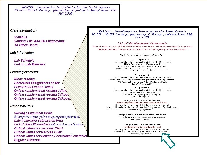
Schedule of readings Before next exam (September 21) Please read chapters 1 - 5 in Open. Stax textbook Please read Appendix D, E & F online On syllabus this is referred to as online readings 1, 2 & 3 Please read Chapters 1, 5, 6 and 13 in. Plous Chapter 1: Selective Perception Chapter 5: Plasticity Chapter 6: Effects of Question Wording and Framing Chapter 13: Anchoring and Adjustment

Random sampling vs Random assignment of participants into groups: Already have Any subject had an equal chance of getting assigned toparticipants either condition (related to quasi versus true experiment) Random sampling of participants into experiment: Each person in the population has an equal chance of being selected to be in the sample Recruiting participants Population: The entire group of people about whom a researcher wants to learn Sample: The subgroup of people who actually participate in a research study

Simple random sampling: each person from the population has an equal probability of being included Sample frame = how you define population Question: Average weight of U of A football player Sample frame population of the U of A football team =RANDBETWEEN(1, 83) 64 Pick 64 th name on the list (64 is just an example here) Let’s take a sample …a random sample 2018

Systematic random sampling: A probability sampling technique that involves selecting every kth person from a sampling frame You pick the number Other examples of systematic random sampling 1) Check every 2000 th light bulb 2) Survey every 10 th voter 3) Sample every 100 th shipping crate

Stratified sampling: sampling technique that involves dividing a sample into subgroups (or strata) and then selecting samples from each of these groups - sampling technique can maintain ratios for the different groups Average number of speeding 12% of sample is from California tickets 7% of sample is from Texas 6% of sample is from Florida 6% from New York 4% from Illinois Average cost for text books for a 4% from Ohio 17. 7% of sample are Pre-business majors semester 4% from Pennsylvania 4. 6% of sample are Psychology majors 3% from Michigan 2. 8% of sample are Biology majors etc 2. 4% of sample are Architecture majors etc

Cluster sampling: sampling technique divides a population sample into subgroups (or clusters) by region or physical space. Can either measure everyone or select samples for each cluster Textbook prices Southwest schools Midwest schools Northwest schools etc Average student income, survey by Old main area Near Mc. Clelland Around Main Gate etc Patient satisfaction for hospital 7 th floor (near maternity ward) 5 th floor (near physical rehab) 2 nd floor (near trauma center) etc

Non-random sampling is vulnerable to bias Convenience sampling: sampling technique that involves sampling people nearby. A non-random sample and vulnerable to bias Snowball sampling: a non-random technique in which one or more members of a population are located and used to lead the researcher to other members of the population Used when we don’t have any other way of finding them - also vulnerable to biases Judgment sampling: sampling technique that involves sampling people who an expert says would be useful. A non-random sample and vulnerable to bias

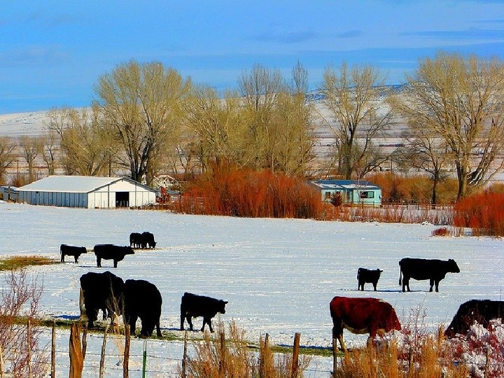
IV: Nominal Ordinal Type of Independent Interval or Mariska works at a cattle ranch, and wants Cow Chow Variable? Ratio? IV: cattle to gain as much weight as possible. Discrete Continuous No, only Random Mariska wants to know if the new feed makes a or discrete? Random convenience Sampling? DV: Nominal difference in how much weight the cattle gain. Assignment? sampling Assignment Ratio Ordinal Weight Dependen (True Expt) Interval or t She gathers the first 100 cows that she finds DV: Ratio? Variable? in the meadow, and then randomly assigns those 100 cows into two groups (50 each group) One group gets the new feed for 6 months, while the other group of cattle gets the old feed. She is not looking for any trends over time, but is just looking for a difference between the two types of cow chow (feed). Continuous or discrete? Betweenor Between Participant within? Design Cross Sectionalor Sectional Time Series

Does amount of sleep (4 vs 8 hours) affect class attendance? Selected 350 students who happened to be walking along the mall from 38, 000 undergraduates at U of Washington and randomly assigned students into two groups. What is the independent variable? - Amount of sleep How many levels are there of the IV? - 2 levels (4 hours vs 8 hours) What is the dependent variable? Group 1 gets 4 hours sleep - Class attendance What is population and sample? Note: Parameter would - Population: whole school - Sample: group of 350 students be what we are guessing for the whole school based on these 350 students What is statistic ? Group 2 gets 8 hours sleep - Average class attendance for 350 students Quasi versus true experiment (random assignment)? - True Random sample? - No, not all students equally likely to be on mall

Does gender of the teacher affect test scores for the students in California? Selected 150 students from Santa Monica and then just asked them to report the gender of their teacher. What is the independent variable? - Gender of teacher How many levels are there of the IV? - 2 levels (male vs female teacher) Group 1 gets a female teacher Group 2 gets a male teacher What is the dependent variable? - Test Scores What is population and sample? - Population: California - Sample: group of 150 students from Santa Monica What is statistic ? - Average test score for 150 students Quasi versus true experiment (random assignment)? - No, no random assignment, just used current teacher Random sample? - No – Random sample would require that everyone in California be equally likely to be chosen.

Scatterplot displays relationships between two continuous variables Correlation: Measure of how two variables co-occur and also can be used for prediction Range between -1 and +1 The closer to zero the weaker the relationship and the worse the prediction Positive or negative

Correlation Range between -1 and +1 +1. 00 perfect relationship = perfect predictor +0. 80 strong relationship = good predictor +0. 20 weak relationship = poor predictor 0 no relationship = very poor predictor -0. 20 weak relationship = poor predictor -0. 80 strong relationship = good predictor -1. 00 perfect relationship = perfect predictor

Positive correlation: as values on one variable go up, so do values for the other variable Negative correlation: as values on one variable go up, the values for the other variable go down Height of Mothers by Height of Daughters Positive Correlation Height of Daughters

Positive correlation: as values on one variable go up, so do values for the other variable Negative correlation: as values on one variable go up, the values for the other variable go down Brushing Teeth Brushing teeth by number cavities Negative Correlation Number Cavities

Perfect correlation = +1. 00 or -1. 00 One variable perfectly predicts the other Height in inches and height in feet Positive correlation Speed (mph) and time to finish race Negative correlation

Correlation The more closely the dots approximate a straight line, (the less spread out they are) the stronger the relationship is. Perfect correlation = +1. 00 or -1. 00 One variable perfectly predicts the other No variability in the scatterplot The dots approximate a straight line

Correlation

Correlation does not imply causation Is it possible that they are causally related? Yes, but the correlational analysis does not answer that question What if it’s a perfect correlation – isn’t that causal? Number of Birthdays No, it feels more compelling, but is neutral about causality Number of Birthday Cakes

Positive correlation: as values on one variable go up, so do values for other variable Negative correlation: as values on one variable go up, the values for other variable go down Number of bathrooms in a city and number of crimes committed Positive correlation

Linear vs curvilinear relationship Linear relationship is a relationship that can be described best with a straight line Curvilinear relationship is a relationship that can be described best with a curved line

http: //neyman. stat. uiuc. edu/~stat 100/cuwu/Games. html http: //argyll. epsb. ca/jreed/math 9/strand 4/scatter. Plot. htm Correlation - How do numerical values change? Let’s estimate the correlation coefficient for each of the following r = +1. 0 r = +. 80 r = -1. 0 r = -. 50 r = 0. 0

This shows a strong positive relationship (r = 0. 97) between the price of the house and its eventual sales price r = +0. 97 Description includes: Both variables Strength (weak, moderate, strong) Direction (positive, negative) Estimated value (actual number)

r = +0. 97 r = -0. 48 This shows a moderate negative relationship (r = -0. 48) between the amount of pectin in orange juice and its sweetness Description includes: Both variables Strength (weak, moderate, strong) Direction (positive, negative) Estimated value (actual number)

Description includes: Both variables Strength (weak, moderate, strong) Direction (positive, negative) Estimated value (actual number) r = -0. 91 This shows a strong negative relationship (r = -0. 91) between the distance that a golf ball is hit and the accuracy of the drive

Description includes: Both variables Strength (weak, moderate, strong) Direction (positive, negative) Estimated value (actual number) This shows a moderate positive relationship (r = 0. 61) between the price of the length of stay in a hospital and the number of services provided r = -0. 91 r = 0. 61

r = +0. 97 r = -0. 48 r = -0. 91 r = 0. 61

Bothaxes have real and values numbers listed are labeled 48 52 5660 64 68 72 Height of Mothers (in) Variable name is listed clearly This shows the strong positive (r = +0. 8) relationship between the heights of daughters (in inches) with heights of their mothers (in inches). 48 52 56 60 64 68 72 76 Height of Daughters (inches) Variable name is listed clearly Description includes: Both variables Strength (weak, moderate, strong) Direction (positive, negative) Estimated value (actual number)

Bothaxes have real and values numbers listed are labeled 48 52 5660 64 68 72 Height of Mothers (in) Variable name is listed clearly This shows the strong positive (r = +0. 8) relationship between the heights of daughters (in inches) with heights of their mothers (in inches). 48 52 56 60 64 68 72 76 Height of Daughters (inches) Variable name is listed clearly Description includes: Both variables Strength (weak, moderate, strong) Direction (positive, negative) Estimated value (actual number)

Bothaxes have real and values numbers listed are labeled 48 52 5660 64 68 72 Height of Mothers (in) Variable name is listed clearly This shows the strong positive (r = +0. 8) relationship between the heights of daughters (in inches) with heights of their mothers (in inches). 48 52 56 60 64 68 72 76 Height of Daughters (inches) Variable name is listed clearly Description includes: Both variables Strength (weak, moderate, strong) Direction (positive, negative) Estimated value (actual number)

Bothaxes have real and values numbers listed are labeled 48 52 5660 64 68 72 Height of Mothers (in) Variable name is listed clearly This shows the strong positive (r = +0. 8) relationship between the heights of daughters (in inches) with heights of their mothers (in inches). 48 52 56 60 64 68 72 76 Height of Daughters (inches) Variable name is listed clearly Description includes: Both variables Strength (weak, moderate, strong) Direction (positive, negative) Estimated value (actual number)

Bothaxes have real and values numbers listed are labeled 48 52 5660 64 68 72 Height of Mothers (in) Variable name is listed clearly This shows the strong positive (r = +0. 8) relationship between the heights of daughters (in inches) with heights of their mothers (in inches). 48 52 56 60 64 68 72 76 Height of Daughters (inches) Variable name is listed clearly Description includes: Both variables Strength (weak, moderate, strong) Direction (positive, negative) Estimated value (actual number)

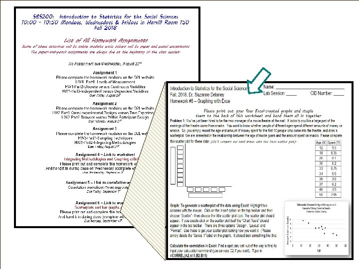
n o i at l e r or ow C n s i t h n t shee i nd ork a H W