Screen Alyson Lecturers desk Row A Chris Row


 Please read chapters 1 - 5")
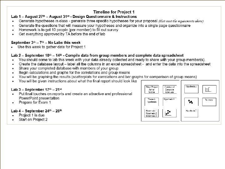


- Slides: 41
Screen Alyson Lecturer’s desk Row A Chris Row C Row B Row A 15 14 12 11 10 13 20 Row B 19 24 23 22 21 Row C 20 19 28 27 26 25 24 23 Row D 22 21 20 19 30 29 28 27 26 25 24 23 Row E 23 22 21 20 19 35 34 33 32 31 30 29 28 27 26 Row F 25 35 34 33 32 31 30 29 28 27 26 Row G 37 36 35 34 33 32 31 30 29 28 41 40 39 38 37 36 35 34 33 32 31 30 25 Row D Row E Row F Row G Row H Row L 33 31 29 23 22 21 Tr ey 21 8 7 6 5 Row A 2 1 3 2 Row B 8 7 6 5 4 12 11 10 9 8 7 6 5 4 3 2 1 24 23 22 21 20 19 18 17 16 15 14 13 12 11 10 9 8 7 6 5 4 3 2 25 24 23 22 21 20 19 18 17 16 15 14 13 12 11 10 9 8 7 6 5 4 3 2 Row H 27 26 25 24 23 22 21 20 19 18 17 16 15 14 13 12 29 Row J 28 27 26 25 24 23 22 21 20 19 18 17 16 15 14 13 12 11 10 9 8 7 6 5 4 3 2 1 Row J 29 Row K 28 27 26 25 24 23 22 21 20 19 18 17 16 15 14 13 12 11 10 9 8 7 6 5 4 3 2 1 Row K 25 Row L 24 23 22 21 20 19 18 17 16 15 14 13 12 11 10 9 20 19 Row M 18 4 3 Row N 15 14 13 12 11 10 9 8 7 6 5 4 3 2 1 Row P 15 14 13 12 11 10 9 8 7 6 5 4 3 2 1 4 3 18 17 18 16 17 15 16 18 14 15 17 18 13 14 13 16 17 12 11 10 15 16 14 15 13 12 11 10 14 17 16 15 14 13 12 11 10 9 13 8 7 6 5 table 14 13 12 11 10 9 8 7 6 Projection Booth Harvill 150 renumbered 3 4 9 32 31 30 29 28 27 26 Row M 9 5 2 1 1 Row C Row D Row E o Fl 1 Row F 1 Row G 11 10 9 8 7 6 5 4 3 2 2 1 1 1 Row L Row M Jun 1 Left handed desk Row H
e v a h u o y f i d e r Even e t s i g e r t e y n a c t o u n o y r e k c i l c r e u t a yo p i c i t r a p still The Gre e She n ets
Introduction to Statistics for the Social Sciences SBS 200 - Lecture Section 001, Fall 2018 Room 150 Harvill Building 10: 00 - 10: 50 Mondays, Wednesdays & Fridays. http: //www. youtube. com/watch? v=o. SQJP 40 Pc. GI
Everyone will want to be enrolled in one of the lab sessions e u n i t n o k c e e s b w La this
Schedule of readings Before next exam (September 21) Please read chapters 1 - 5 in Open. Stax textbook Please read Appendix D, E & F online On syllabus this is referred to as online readings 1, 2 & 3 Please read Chapters 1, 5, 6 and 13 in. Plous Chapter 1: Selective Perception Chapter 5: Plasticity Chapter 6: Effects of Question Wording and Framing Chapter 13: Anchoring and Adjustment
Overview Frequency distributions The normal curve Challenge yourself as we work through characteristics of distributions to try to categorize each concept as a measure of 1) central tendency 2) dispersion or 3) shape Mean, Median, Mode, Trimmed Mean Skewed right, skewed left unimodal, bimodal, symmetric
Dot Plot R w e i ev
Let’s create a distribution of the baseball players in the University of Arizona Baseball team Diallo is 6’ 0” Diallo 5’ 8” 5’ 10” 6’ 2” 6’ 4” R w e i ev
Let’s create a distribution of the baseball players in the University of Arizona Baseball team Diallo is 6’ 0” Preston is 6’ 2” Preston 5’ 8” 5’ 10” 6’ 2” 6’ 4” R w e i ev
Let’s create a distribution of the baseball players in the University of Arizona Baseball team Diallo is 6’ 0” Preston is 6’ 2” Hunter Mike is 5’ 8” Mike 5’ 8” Hunter is 5’ 10” 6’ 2” 6’ 4” R w e i ev
Let’s create a distribution of the baseball players in the University of Arizona Baseball team Diallo is 6’ 0” Preston is 6’ 2” Mike is 5’ 8” Hunter is 5’ 10” Shea is 6’ 4” 5’ 8” 5’ 10” 6’ 2” 6’ 4” David is 6’ 0” R w e i ev
Let’s create a distribution of the baseball players in the University of Arizona Baseball team R w e i ev
Measure of central tendency: describes how scores tend to cluster toward the center of the distribution Normal distribution In all distributions: mode = tallest point median = middle score mean = balance point In a normal distribution: mode = mean = median R w e i ev
Measure of central tendency: describes how scores tend to cluster toward the center of the distribution Positively skewed distribution In all distributions: mode = tallest point median = middle score mean = balance point In a positively skewed distribution: mode < median < mean Note: mean is most affected by outliers or skewed distributions
Measure of central tendency: describes how scores tend to cluster toward the center of the distribution Negatively skewed distribution In all distributions: mode = tallest point median = middle score mean = balance point In a negatively skewed distribution: mean < median < mode Note: mean is most affected by outliers or skewed distributions
Mode: The value of the most frequent observation Bimodal distribution: Distribution with two most frequent observations (2 peaks) Example: Ian coaches two boys baseball teams. One team is made up of 10 -year-olds and the other is made up of 16 -year-olds. When he measured the height of all of his players he found a bimodal distribution
Frequency Remember… 10 20 30 Note: Always “frequency” 40 50 60 70 80 Score on Exam 90 100 Note: Label and Numbers
Overview Frequency distributions The normal curve Challenge yourself as we work through characteristics of distributions to try to categorize each concept as a measure of 1) central tendency 2) dispersion or 3) shape Mean, Median, Mode, Trimmed Mean Standard deviation, Variance, Range Mean Absolute Deviation Skewed right, skewed left unimodal, bimodal, symmetric
Variability Some distributions are more variable than others 5’ 5’ 6” 6’ 6’ 6” 7’ What might this be? Let’s say this is our distribution of heights of men on U of A baseball team Mean is 6 feet tall What might this be? 5’ 5’ 6” 6’ 6’ 6” 7’
Dispersion: Variability Some distributions are more variable than others A 5’ 5’ 6” 6’ 6’ 6” 7’ Range: The difference between the largest and smallest observations Range for distribution A? B Range for distribution B? 5’ 5’ 6” 6’ 6’ 6” 7’ C 5’ Range for distribution C? The larger the variability the wider the curve tends to be 5’ 6” 6’ 6’ 6” 7’ The smaller the variability the narrower the curve tends to be
Variability 5’ 5’ 6” 6’ 6’ 6” 7’ 7’ 7’ The larger the variability the wider the curve the larger the deviations scores tend to be The smaller the variability the narrower the curve the smaller the deviations scores tend to be But what is a “deviation score”?
Deviation scores Diallo is 0” Distribution of the baseball players: Deviation scores Diallo is 6’ 0” Diallo’s deviation score is 0 6’ 0” – 6’ 0” = 0 Diallo 5’ 8” 5’ 10” 6’ 2” 6’ 4”
Deviation scores Distribution of the baseball players: Deviation scores Diallo is 0” Preston is 2” Diallo is 6’ 0” Diallo’s deviation score is 0 Preston is 6’ 2” Preston 5’ 8” 5’ 10” 6’ 2” Preston’s deviation score is 2” 6’ 2” – 6’ 0” = 2 6’ 4”
Deviation scores Distribution of the baseball players: Deviation scores Diallo is 0” Preston is 2” Mike is -4” Hunter is -2 Diallo is 6’ 0” Diallo’s deviation score is 0 Hunter Preston is 6’ 2” Preston’s deviation score is 2” Mike is 5’ 8” Mike’s deviation score is -4” 5’ 8” 5’ 10” 6’ 2” 6’ 4” 5’ 8” – 6’ 0” = -4 Hunter is 5’ 10” Hunter’s deviation score is -2” 5’ 10” – 6’ 0” = -2
Deviation scores Distribution of the baseball players: Deviation scores David Shea Diallo is 0” Preston is 2” Mike is -4” Hunter is -2 Shea is 4 David is 0” Diallo’s deviation score is 0 Preston’s deviation score is 2” Mike’s deviation score is -4” Hunter’s deviation score is -2” Shea is 6’ 4” 5’ 8” 5’ 10” 6’ 2” 6’ 4” Shea’s deviation score is 4” 6’ 4” – 6’ 0” = 4 David is 6’ 0” David’s deviation score is 0 6’ 0” – 6’ 0” = 0
Deviation scores Distribution of the baseball players: Deviation scores David Shea Diallo is 0” Preston is 2” Mike is -4” Hunter is -2 Shea is 4 David is 0” Diallo’s deviation score is 0 Preston’s deviation score is 2” Mike’s deviation score is -4” Hunter’s deviation score is -2” Shea’s deviation score is 4” David’s deviation score is 0” 5’ 8” 5’ 10” 6’ 2” 6’ 4”
Deviation scores Distribution of the baseball players: Deviation scores 5’ 8” 5’ 10” 6’ 2” 6’ 4” Diallo is 0” Preston is 2” Mike is -4” Hunter is -2 Shea is 4 David is 0”
Deviation scores Distribution of the baseball players: Deviation scores 5’ 8” 5’ 10” 6’ 2” 6’ 4” Diallo is 0” Preston is 2” Mike is -4” Hunter is -2 Shea is 4 David is 0”
Deviation scores Distribution of the baseball players: Deviation scores 5’ 8” 5’ 10” 6’ 2” 6’ 4” Diallo is 0” Preston is 2” Mike is -4” Hunter is -2 Shea is 4 David is 0”
Deviation scores How to find the average deviation Diallo is 0” Preston is 2” Mike is -4” Hunter is -2 Shea is 4 David is 0” Mike Hunter 5’ 8” 5’ 10” 6’ 2” 6’ 4” How do we find the average height? Σx = average height N How do we find the average spread? Preston Σ(x - µ) = average deviation N Σ (x - µ) = ? 5’ 8” 5’ 9” 5’ 10’ 5’ 11” 6’ 0” 6’ 1” 6’ 2” 6’ 3” 6’ 4” - 6’ 0” = - 4” 6’ 0” = - 3” 6’ 0” = - 2” 6’ 0” = - 1” 6’ 0 = 0 6’ 0” = + 1” 6’ 0” = + 2” 6’ 0” = + 3” 6’ 0” = + 4” Σ(x - x) = 0 Σ(x - µ) = 0 Diallo
Deviation scores How to find the average deviation Diallo is 0” Preston is 2” Mike is -4” Hunter is -2 Shea is 4 David is 0” Σx- x=? 5’ 8” Big proble m 5’ 10” 6’ 2” 6’ 4” This is called “sum of Square the squares” deviations Σx N 2 Σ(x - µ) N 2 Σ(x - x) 2 Σ(x - µ) 5’ 8” 5’ 9” 5’ 10’ 5’ 11” 6’ 0” 6’ 1” 6’ 2” 6’ 3” 6’ 4” - 6’ 0” = - 4” 6’ 0” = - 3” 6’ 0” = - 2” 6’ 0” = - 1” 6’ 0 = 0 6’ 0” = + 1” 6’ 0” = + 2” 6’ 0” = + 3” Big 6’ 0” = + 4” proble - x) = 0 m Σ(x - µ) = 0
How to find the average deviation Mean: The average value in the data Standard deviation: The average amount scores deviate on either side of their mean Mean is a measure of typical “value” (where the typical scores are positioned on the number line) Standard deviation is typical “spread” or typical size of deviations or distance from mean – can never be negative
Standard deviation: The average amount by which observations deviate on either side of their mean These would be helpful to know by heart – please memorize these formula
Standard deviation: The average amount by which observations deviate on either side of their mean What do these two formula have in common? d dar n a t S e ianc r : t a c v Fa d = e r Fun a squ n o i t devia
Standard deviation: The average amount by which observations deviate on either side of their mean Note this is for population standard deviation & variance What do these two formula have in common? Note this is for sample standard deviation & variance
Standard deviation: The average amount by which observations deviate on either side of their mean “Sum of Squares” You know by heart – you’ve memorized these formula
Standard deviation: The average amount by which observations deviate on either side of their mean “degrees of freedom” You know by heart – you’ve memorized these formula
Standard deviation: The average amount by which observations deviate on either side of their mean Deviation scores Diallo is 0” Preston is 2” Mike is -4” Hunter is -2 Shea is 4 David 0” Remember, it’s relative to the mean Generally, (on average) how far away is each score from the mean? Based on difference from the mean Please memorize these Mean Diallo Mike Preston Shea