Screen Stage Lecturers desk Row C Row D

Screen Stage Lecturer’s desk Row C Row D Row E Row F Row G Row H Row J Row K Row L Row M 28 27 26 28 27 25 24 23 22 26 25 24 23 22 28 27 26 25 24 23 22 28 27 26 25 24 23 22 28 27 26 25 24 23 22 table 3 broke n desk 2 1 Row A Row B Row C Row D Row E Row F Row G Row H Row J Row K Row L Row M 14 13 12 11 10 9 8 7 6 5 4 3 2 1 21 20 19 18 17 16 15 14 13 12 11 10 9 8 7 6 5 4 3 2 1 21 20 19 18 17 16 15 14 13 12 11 10 9 8 7 6 5 4 3 2 1 21 20 19 18 17 16 15 14 13 12 11 10 9 8 7 6 5 4 3 2 1 21 20 19 18 17 16 13 12 11 10 9 8 7 6 5 4 3 2 1 14 13 2 1 Projection Booth Modern Languages R/L handed table 3 2 1 Row C Row D Row E Row F Row G Row H Row J Row K Row L Row M

MGMT 276: Statistical Inference in Management Spring 2015

Schedule of readings Before our fourth exam (April 30 th) Lind Chapter 13: Linear Regression and Correlation Chapter 14: Multiple Regression Chapter 15: Chi-Square Plous Chapter 17: Social Influences Chapter 18: Group Judgments and Decisions

Over next couple of lectures 4/21/15 Logic of hypothesis testing with Correlations Interpreting the Correlations and scatterplots Simple and Multiple Regression Using correlation for predictions r versus r 2 Regression uses the predictor variable (independent) to make predictions about the predicted variable (dependent) Coefficient of correlation is name for “r” Coefficient of determination is name for “r 2” (remember it is always positive – no direction info) Standard error of the estimate is our measure of the variability of the dots around the regression line (average deviation of each data point from the regression line – like standard deviation) Coefficient of regression will “b” for each variable (like slope)

Homework due – Thursday (April 23 rd) On class website: Please print and complete homeworksheet #17 Multiple Regression Analyses

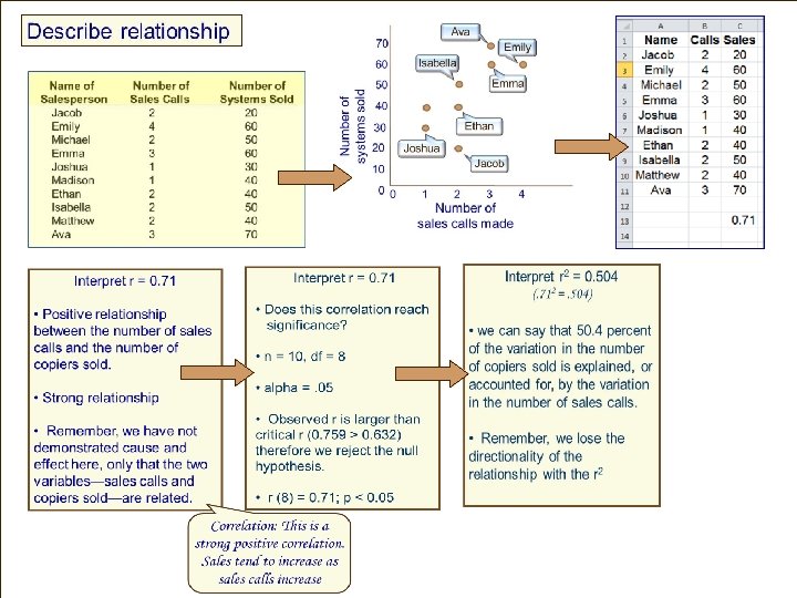
Regression Example Rory is an owner of a small software company and employs 10 sales staff. Rory send his staff all over the world consulting, selling and setting up his system. He wants to evaluate his staff in terms of who are the most (and least) productive sales people and also whether more sales calls actually result in more systems being sold. So, he simply measures the number of sales calls made by each sales person and how many systems they successfully sold.

Regression Example Step 1: Draw scatterplot Step 2: Estimate r 70 60 Number of systems sold Do more sales calls result in more sales made? Ava Dependent Variable Emily Isabella Emma 50 40 Ethan 30 20 Joshua Jacob 10 0 0 1 2 3 4 Number of sales calls made Independent Variable

Regression Example Do more sales calls result in more sales made? Step 3: Calculate r Step 4: Is it a significant correlation?

Do more sales calls result in more sales made? Step 4: Is it a significant correlation? • n = 10, df = 8 • alpha =. 05 • Observed r is larger than critical r Step 3: Calculate r • (0. 71 > 0. 632) • therefore we reject the null hypothesis. Step Is it a significant • Yes it is 4: a significant correlation? • r (8) = 0. 71; p < 0. 05

Regression: Predicting sales Step 1: Draw prediction line r = 0. 71 b = 11. 579 (slope ) a = 20. 526 (intercept) Draw a regression line and regression equation What are w e predicting?

Regression: Predicting sales Step 1: Draw prediction line r = 0. 71 b = 11. 579 (slope ) a = 20. 526 (intercept) Draw a regression line and regression equation

Regression: Predicting sales Step 1: Draw prediction line r = 0. 71 b = 11. 579 (slope ) a = 20. 526 (intercept) Draw a regression line and regression equation

Regression: Predicting sales Step 1: Predict sales for a certain number of sales calls You should sell 32. 105 systems Step 2: State the regression equation Y’ = a + bx Y’ = 20. 526 + 11. 579 x Step 3: Solve for some value of Y’ Y’ = 20. 526 + 11. 579(1) Y’ = 32. 105 What should you expect from a salesperson who makes 1 calls? They should sell 32. 105 systems If they sell more over performing If they sell fewer underperforming Madison Joshua If make one sales call

Regression: Predicting sales Step 1: Predict sales for a certain number of sales calls Step 2: State the regression equation Y’ = a + bx Y’ = 20. 526 + 11. 579 x Step 3: Solve for some value of Y’ Y’ = 20. 526 + 11. 579(2) Y’ = 43. 684 What should you expect from a salesperson who makes 2 calls? They should sell 43. 68 systems If they sell more over performing If they sell fewer underperforming You should sell Isabella 43. 684 systems Jacob If make two sales call

Regression: Predicting sales Step 1: Predict sales for a certain number of sales calls You should sell 55. 263 systems Step 2: State the regression equation Y’ = a + bx Y’ = 20. 526 + 11. 579 x Step 3: Solve for some value of Y’ Y’ = 20. 526 + 11. 579(3) Y’ = 55. 263 What should you expect from a salesperson who makes 3 calls? They should sell 55. 263 systems If they sell more over performing If they sell fewer underperforming Ava Emma If make three sales call

Regression: Predicting sales Step 1: Predict sales for a certain number of sales calls You should sell 66. 84 systems Step 2: State the regression equation Y’ = a + bx Y’ = 20. 526 + 11. 579 x Step 3: Solve for some value of Y’ Y’ = 20. 526 + 11. 579(4) Y’ = 66. 842 What should you expect from a salesperson who makes 4 calls? They should sell 66. 84 systems If they sell more over performing If they sell fewer underperforming Emily If make four sales calls

Regression: Evaluating Staff Step 1: Compare expected sales levels to actual sales levels Ava Isabella Emma Emily Madison Joshua Jacob What should you expect from each salesperson They should sell x systems depending on sales calls If they sell more over performing If they sell fewer underperforming

Regression: Evaluating Staff Step 1: Compare expected sales levels to actual sales levels 70 -55. 3=14. 7 Ava 14. 7 Difference between expected Y’ and actual Y is called “residual” (it’s a deviation score) How did Ava do? Ava sold 14. 7 more than expected taking into account how many sales calls she made over performing

Regression: Evaluating Staff Step 1: Compare expected sales levels to actual sales levels 20 -43. 7=-23. 7 Difference between expected Y’ and actual Y is called “residual” (it’s a deviation score) Ava -23. 7 Jacob How did Jacob do? Jacob sold 23. 684 fewer than expected taking into account how many sales calls he made under performing

Regression: Evaluating Staff Step 1: Compare expected sales levels to actual sales levels Ava Isabella Emma Emily Madison Joshua Jacob What should you expect from each salesperson They should sell x systems depending on sales calls If they sell more over performing If they sell fewer underperforming

Regression: Evaluating Staff Step 1: Compare expected sales levels to actual sales levels Ava Isabella Madison 14. 7 Emma -6. 8 -23. 7 7. 9 Joshua Jacob Difference between expected Y’ and actual Y is called “residual” (it’s a deviation score) Emily

Does the prediction line perfectly the predicted variable when using the predictor variable? No, we are wrong sometimes… How can we estimate how much “error” we have? Exactly? 14. 7 -23. 7 Difference between expected Y’ and actual Y is called “residual” (it’s a deviation score) How would we find our “average residual”? The green lines show much “error” there is in our prediction line…how much we are wrong in our predictions

How do we find the average amount of error in our prediction The average amount by which actual scores deviate on either side of the predicted score Residual scores Ava is 14. 7 Jacob is -23. 7 Emily is -6. 8 Madison is 7. 9 Step 1: Find error for each value (just the residuals) Y – Y’ Step 2: Add up the residuals Σ(Y – Y’) = 0 Σ(Y – Square root Y’) 2 Big problem Square the deviations Σ(Y – Y’) 2 n-2 Divide by df Difference between expected Y’ and actual Y is called “residual” (it’s a deviation score) How would we find our “average residual”? Σx N The green lines show much “error” there is in our prediction line…how much we are wrong in our predictions

Standard error of the estimate (line) = These would be helpful to know by heart – please memorize these formula

How well does the prediction line predict the predicted variable when using the predictor variable? Standard error of the estimate (line) What if we want to know the “average deviation score”? Finding the standard error of the estimate (line) Standard error of the estimate: • a measure of the average amount of predictive error • the average amount that Y’ scores differ from Y scores • a mean of the lengths of the green lines • Slope doesn’t give “variability” info • Intercept doesn’t give “variability info • Correlation “r” does give “variability info • Residuals do give “variability info

How well does the prediction line predict the Ys from the Xs? A note about curvilinear relationships and patterns of the residuals Residuals • Shorter green lines suggest better prediction – smaller error • Longer green lines suggest worse prediction – larger error • Why are green lines vertical? Remember, we are predicting the variable on the Y axis So, error would be how we are wrong about Y (vertical)

Does the prediction line perfectly the predicted variable when using the predictor variable? No, we are wrong sometimes… How can we estimate how much “error” we have? 14. 7 -23. 7 Difference between expected Y’ and actual Y is called “residual” (it’s a deviation score) The green lines show much “error” there is in our prediction line…how much we are wrong in our predictions Perfect correlation = +1. 00 or -1. 00 Each variable perfectly predicts the other No variability in the scatterplot The dots approximate a straight line

Regression Analysis – Least Squares Principle When we calculate the regression line we try to: • minimize distance between predicted Ys and actual (data) Y points (length of green lines) • remember because of the negative and positive values cancelling each other out we have to square those distance (deviations) • so we are trying to minimize the “sum of squares of the vertical distances between the actual Y values and the predicted Y values”

Is the regression line better than just guessing the mean of the Y variable? How much does the information about the relationship actually help? Which minimizes error better? How much better does the regression line predict the observed results? 2 r o W ! w

What is r 2? r 2 = The proportion of the total variance in one variable that is predictable by its relationship with the other variable Examples If mother’s and daughter’s heights are correlated with an r =. 8, then what amount (proportion or percentage) of variance of mother’s height is accounted for by daughter’s height? . 64 because (. 8)2 =. 64

What is r 2? r 2 = The proportion of the total variance in one variable that is predictable for its relationship with the other variable Examples If mother’s and daughter’s heights are correlated with an r =. 8, then what proportion of variance of mother’s height is not accounted for by daughter’s height? . 36 because (1. 0 -. 64) =. 36 or 36% because 100% - 64% = 36%

What is r 2? r 2 = The proportion of the total variance in one variable that is predictable for its relationship with the other variable Examples If ice cream sales and temperature are correlated with an r =. 5, then what amount (proportion or percentage) of variance of ice cream sales is accounted for by temperature? . 25 because (. 5)2 =. 25

What is r 2? r 2 = The proportion of the total variance in one variable that is predictable for its relationship with the other variable Examples If ice cream sales and temperature are correlated with an r =. 5, then what amount (proportion or percentage) of variance of ice cream sales is not accounted for by temperature? . 75 because (1. 0 -. 25) =. 75 or 75% because 100% - 25% = 75%

Some useful terms • Regression uses the predictor variable (independent) to make predictions about the predicted variable (dependent) • • Coefficient of correlation is name for “r” Coefficient of determination is name for “r 2” (remember it is always positive – no direction info) • Standard error of the estimate is our measure of the variability of the dots around the regression line (average deviation of each data point from the regression line – like standard deviation)

Summary Intercept: suggests that we can assume each salesperson will sell at least 20. 526 systems Slope: as sales calls increase by one, 11. 579 more systems should be sold

Homework Review

Multiple regression equations Can use variables to predict • behavior of stock market • probability of accident • amount of pollution in a particular well • quality of a wine for a particular year • which candidates will make best workers

Can use variables to predict which candidates will make best workers • Measured current workers – the best workers tend to have highest “success scores”. (Success scores range from 1 – 1, 000) • Try to predict which applicants will have the highest success score. • We have found that these variables predict success: • Age (X 1) Both 10 point scales • Niceness (X 2) Niceness (10 = really nice) Harshness (10 = really harsh) • Harshness (X 3) According to your research, age has only a small effect on success, while workers’ attitude has a big effect. Turns out, the best workers have high “niceness” scores and low “harshness” scores. Your results are summarized by this regression formula: Y’ = b 1 X 1+ b 2 X 2+ b 3 X 3 + a Y’ = b 1 X 1 + b 2 Success score = X 2 + b 3 X 3 +a (1)(Age) + (20)(Nice) + (-75)(Harsh) + 700

According to your research, age has only a small effect on success, while workers’ attitude has a big effect. Turns out, the best workers have high “niceness” scores and low “harshness” scores. Your results are summarized by this regression formula: Y’ = b 1 X 1 + b 2 Success score = X 2 + b 3 X 3 +a (1)(Age) + (20)(Nice) + (-75)(Harsh) + 700

According to your research, age has only a small effect on success, while workers’ attitude has a big effect. Turns out, the best workers have high “niceness” scores and low “harshness” scores. Your results are summarized by this regression formula: Y’ = b 1 X 1 + b 2 X 2 + b 3 X 3 + a Success score = (1)(Age) + (20)(Nice) + (-75)(Harsh) + 700 • Y’ is the dependent variable • “Success score” is your dependent variable. • X 1 X 2 and X 3 are the independent variables • “Age”, “Niceness” and “Harshness” are the independent variables. • Each “b” is called a regression coefficient. • Each “b” shows the change in Y for each unit change in its own X (holding the other independent variables constant). • a is the Y-intercept

Y’ = b 1 X 1 + b 2 X 2 + b 3 X 3+ a The Multiple Regression Equation – Interpreting the Regression Coefficients Success score = (1)(Age) + (20)(Nice) + (-75)(Harsh) + 700 b 1 = The regression coefficient for age (X 1) is “ 1” The coefficient is positive and suggests a positive correlation between age and success. As the age increases the success score increases. The numeric value of the regression coefficient provides more information. If age increases by 1 year and hold the other two independent variables constant, we can predict a 1 point increase in the success score. 14 -45

Y’ = b 1 X 1 + b 2 X 2 + b 3 X 3+ a The Multiple Regression Equation – Interpreting the Regression Coefficients Success score = (1)(Age) + (20)(Nice) + (-75)(Harsh) + 700 b 2 = The regression coefficient for age (X 2) is “ 20” The coefficient is positive and suggests a positive correlation between niceness and success. As the niceness increases the success score increases. The numeric value of the regression coefficient provides more information. If the “niceness score” increases by one, and hold the other two independent variables constant, we can predict a 20 point increase in the success score. 14 -46

Y’ = b 1 X 1 + b 2 X 2 + b 3 X 3+ a The Multiple Regression Equation – Interpreting the Regression Coefficients Success score = (1)(Age) + (20)(Nice) + (-75)(Harsh) + 700 b 3 = The regression coefficient for age (X 3) is “-75” The coefficient is negative and suggests a negative correlation between harshness and success. As the harshness increases the success score decreases. The numeric value of the regression coefficient provides more information. 14 -47 If the “harshness score” increases by one, and hold the other two independent variables constant, we can predict a 75 point decrease in the success score.