Screen Lecturers desk Row A Row B Row

Screen Lecturer’s desk Row A Row B Row A 15 14 12 11 10 13 20 Row B 19 24 23 22 21 Row C 20 19 28 27 26 25 24 23 Row D 22 21 20 19 30 29 28 27 26 25 24 23 Row E 23 22 21 20 19 35 34 33 32 31 30 29 28 27 26 Row F 25 35 34 33 32 31 30 29 28 27 26 Row G 37 36 35 34 33 32 31 30 29 28 41 40 39 38 37 36 35 34 33 32 31 30 Row C Row D Row E Row F Row G Row H Row L 33 31 29 25 23 22 21 21 8 7 6 5 3 4 Row A 2 1 3 2 Row B 9 8 7 6 5 4 12 11 10 9 8 7 6 5 4 3 2 1 24 23 22 21 20 19 18 17 16 15 14 13 12 11 10 9 8 7 6 5 4 3 2 1 Row F 25 24 23 22 21 20 19 18 17 16 15 14 13 12 11 10 9 8 7 6 5 4 3 2 1 Row G Row H 27 26 25 24 23 22 21 20 19 18 17 16 15 14 13 12 29 Row J 28 27 26 25 24 23 22 21 20 19 18 17 16 15 14 13 12 11 10 9 8 7 6 5 4 3 2 1 Row J 29 Row K 28 27 26 25 24 23 22 21 20 19 18 17 16 15 14 13 12 11 10 9 8 7 6 5 4 3 2 1 Row K 25 Row L 24 23 22 21 20 19 18 17 16 15 14 13 12 11 10 9 20 19 Row M 18 4 3 Row N 15 14 13 12 11 10 9 8 7 6 5 4 3 2 1 Row P 15 14 13 12 11 10 9 8 7 6 5 4 3 2 1 4 3 32 31 30 29 28 27 26 Row M 9 18 17 18 16 17 15 16 18 14 15 17 18 13 14 13 16 17 12 11 10 15 16 14 15 13 12 11 10 14 17 16 15 14 13 12 11 10 9 13 8 7 6 5 table 15 14 13 12 11 10 9 8 7 6 Projection Booth 5 2 1 1 1 Row C Row D Row E 11 10 9 8 7 6 5 4 3 2 2 1 1 1 Row L Row M Harvill 150 renumbered Left handed desk Row H

Screen Kristina Lecturer’s desk Row A Attila Row C Row B Row A 15 14 12 11 10 13 20 Row B 19 24 23 22 21 Row C 20 19 28 27 26 25 24 23 Row D 22 21 20 19 30 29 28 27 26 25 24 23 Row E 23 22 21 20 19 35 34 33 32 31 30 29 28 27 26 Row F 25 35 34 33 32 31 30 29 28 27 26 Row G 37 36 35 34 33 32 31 30 29 28 41 40 39 38 37 36 35 34 33 32 31 30 25 Row D Row E Row F Row G Row H Row L 33 31 29 23 22 21 Ha nn a h 21 8 7 6 5 Row A 2 1 3 2 Row B 8 7 6 5 4 12 11 10 9 8 7 6 5 4 3 2 1 24 23 22 21 20 19 18 17 16 15 14 13 12 11 10 9 8 7 6 5 4 3 2 25 24 23 22 21 20 19 18 17 16 15 14 13 12 11 10 9 8 7 6 5 4 3 2 Row H 27 26 25 24 23 22 21 20 19 18 17 16 15 14 13 12 29 Row J 28 27 26 25 24 23 22 21 20 19 18 17 16 15 14 13 12 11 10 9 8 7 6 5 4 3 2 1 Row J 29 Row K 28 27 26 25 24 23 22 21 20 19 18 17 16 15 14 13 12 11 10 9 8 7 6 5 4 3 2 1 Row K 25 Row L 24 23 22 21 20 19 18 17 16 15 14 13 12 11 10 9 20 19 Row M 18 4 3 Row N 15 14 13 12 11 10 9 8 7 6 5 4 3 2 1 Row P 15 14 13 12 11 10 9 8 7 6 5 4 3 2 1 4 3 18 17 18 16 17 15 16 18 14 15 17 18 13 14 13 16 17 12 11 10 15 16 14 15 13 12 11 10 14 17 16 15 14 13 12 11 10 9 13 8 7 6 5 table 14 13 12 11 10 9 8 7 6 Projection Booth Harvill 150 renumbered 3 4 9 32 31 30 29 28 27 26 Row M 9 5 2 1 1 Row C Row D le l e h. Row F Row E M ic 1 1 Row G 11 10 9 8 7 6 5 4 3 2 2 1 1 1 Row L Row M e Sez n 1 Left handed desk Row H

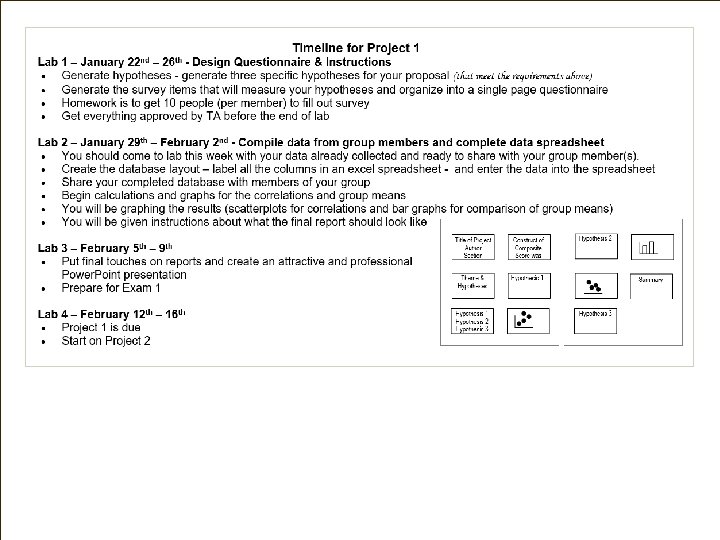
Introduction to Statistics for the Social Sciences SBS 200 - Lecture Section 001, Spring 2018 Room 150 Harvill Building 9: 00 - 9: 50 Mondays, Wednesdays & Fridays. 1/29/18 http: //www. youtube. com/watch? v=o. SQJP 40 Pc. GI

Everyone will want to be enrolled in one of the lab sessions Labs c ontinu e this w eek
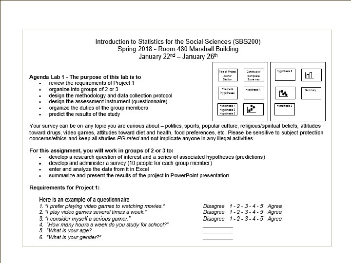

Remember bring your writing assignment forms notebook and clickers to each lecture

In nearly every class we will use clickers to answer questions in class and participate in interactive class demonstrations e v a h u o y f i d e r Even e t s i g e r t e y n a c t o u n o y r e k c i l c r e u t a yo p i c i t r a p still
 Please read chapters 1 - 5")
Schedule of readings Before next exam (February 9) Please read chapters 1 - 5 in Open. Stax textbook Please read Appendix D, E & F online On syllabus this is referred to as online readings 1, 2 & 3 Please read Chapters 1, 5, 6 and 13 in. Plous Chapter 1: Selective Perception Chapter 5: Plasticity Chapter 6: Effects of Question Wording and Framing Chapter 13: Anchoring and Adjustment

Scatterplot displays relationships between two continuous variables Correlation: Measure of how two variables co-occur and also can be used for prediction Range between -1 and +1 The closer to zero the weaker the relationship and the worse the prediction Positive or negative

Correlation Range between -1 and +1 +1. 00 perfect relationship = perfect predictor +0. 80 strong relationship = good predictor +0. 20 weak relationship = poor predictor 0 no relationship = very poor predictor -0. 20 weak relationship = poor predictor -0. 80 strong relationship = good predictor -1. 00 perfect relationship = perfect predictor

Positive correlation: as values on one variable go up, so do values for the other variable Negative correlation: as values on one variable go up, the values for the other variable go down Height of Mothers by Height of Daughters Positive Correlation Height of Daughters

Positive correlation: as values on one variable go up, so do values for the other variable Negative correlation: as values on one variable go up, the values for the other variable go down Brushing Teeth Brushing teeth by number cavities Negative Correlation Number Cavities

Perfect correlation = +1. 00 or -1. 00 One variable perfectly predicts the other Height in inches and height in feet Positive correlation Speed (mph) and time to finish race Negative correlation

Correlation The more closely the dots approximate a straight line, (the less spread out they are) the stronger the relationship is. Perfect correlation = +1. 00 or -1. 00 One variable perfectly predicts the other No variability in the scatterplot The dots approximate a straight line

Correlation

Correlation does not imply causation Is it possible that they are causally related? Yes, but the correlational analysis does not answer that question What if it’s a perfect correlation – isn’t that causal? Number of Birthdays No, it feels more compelling, but is neutral about causality Number of Birthday Cakes

Positive correlation: as values on one variable go up, so do values for other variable Negative correlation: as values on one variable go up, the values for other variable go down Number of bathrooms in a city and number of crimes committed Positive correlation

Linear vs curvilinear relationship Linear relationship is a relationship that can be described best with a straight line Curvilinear relationship is a relationship that can be described best with a curved line

http: //neyman. stat. uiuc. edu/~stat 100/cuwu/Games. html http: //argyll. epsb. ca/jreed/math 9/strand 4/scatter. Plot. htm Correlation - How do numerical values change? Let’s estimate the correlation coefficient for each of the following r = +1. 0 r = +. 80 r = -1. 0 r = -. 50 r = 0. 0
 between the price of")
This shows a strong positive relationship (r = 0. 97) between the price of the house and its eventual sales price r = +0. 97 Description includes: Both variables Strength (weak, moderate, strong) Direction (positive, negative) Estimated value (actual number)

r = +0. 97 r = -0. 48 This shows a moderate negative relationship (r = -0. 48) between the amount of pectin in orange juice and its sweetness Description includes: Both variables Strength (weak, moderate, strong) Direction (positive, negative) Estimated value (actual number)
 Direction (positive, negative) Estimated value (actual")
Description includes: Both variables Strength (weak, moderate, strong) Direction (positive, negative) Estimated value (actual number) r = -0. 91 This shows a strong negative relationship (r = -0. 91) between the distance that a golf ball is hit and the accuracy of the drive
 Direction (positive, negative) Estimated value (actual")
Description includes: Both variables Strength (weak, moderate, strong) Direction (positive, negative) Estimated value (actual number) This shows a moderate positive relationship (r = 0. 61) between the price of the length of stay in a hospital and the number of services provided r = -0. 91 r = 0. 61

r = +0. 97 r = -0. 48 r = -0. 91 r = 0. 61

Bothaxes have real and values numbers listed are labeled 48 52 5660 64 68 72 Height of Mothers (in) Variable name is listed clearly This shows the strong positive (r = +0. 8) relationship between the heights of daughters (in inches) with heights of their mothers (in inches). 48 52 56 60 64 68 72 76 Height of Daughters (inches) Variable name is listed clearly Description includes: Both variables Strength (weak, moderate, strong) Direction (positive, negative) Estimated value (actual number)

Bothaxes have real and values numbers listed are labeled 48 52 5660 64 68 72 Height of Mothers (in) Variable name is listed clearly This shows the strong positive (r = +0. 8) relationship between the heights of daughters (in inches) with heights of their mothers (in inches). 48 52 56 60 64 68 72 76 Height of Daughters (inches) Variable name is listed clearly Description includes: Both variables Strength (weak, moderate, strong) Direction (positive, negative) Estimated value (actual number)

Bothaxes have real and values numbers listed are labeled 48 52 5660 64 68 72 Height of Mothers (in) Variable name is listed clearly This shows the strong positive (r = +0. 8) relationship between the heights of daughters (in inches) with heights of their mothers (in inches). 48 52 56 60 64 68 72 76 Height of Daughters (inches) Variable name is listed clearly Description includes: Both variables Strength (weak, moderate, strong) Direction (positive, negative) Estimated value (actual number)

Bothaxes have real and values numbers listed are labeled 48 52 5660 64 68 72 Height of Mothers (in) Variable name is listed clearly This shows the strong positive (r = +0. 8) relationship between the heights of daughters (in inches) with heights of their mothers (in inches). 48 52 56 60 64 68 72 76 Height of Daughters (inches) Variable name is listed clearly Description includes: Both variables Strength (weak, moderate, strong) Direction (positive, negative) Estimated value (actual number)

Bothaxes have real and values numbers listed are labeled 48 52 5660 64 68 72 Height of Mothers (in) Variable name is listed clearly This shows the strong positive (r = +0. 8) relationship between the heights of daughters (in inches) with heights of their mothers (in inches). 48 52 56 60 64 68 72 76 Height of Daughters (inches) Variable name is listed clearly Description includes: Both variables Strength (weak, moderate, strong) Direction (positive, negative) Estimated value (actual number)

Break into groups of 2 or 3 Each person hand in own worksheet. Be sure to list your name and names of all others in your group Use examples that are different from those is lecture 1. Describe one positive correlation Draw a scatterplot (label axes) 2. Describe one negative correlation Draw a scatterplot (label axes) 3. Describe one zero correlation Draw a scatterplot (label axes) You h a 12 mi ve nutes (appr oxim minut ately r exa 2 mple es pe ) 4. Describe one perfect correlation (positive or negative) Draw a scatterplot (label axes) 5. Describe curvilinear relationship Draw a scatterplot (label axes)

Bothaxes have real and values numbers listed are labeled 48 52 5660 64 68 72 Height of Mothers (in) Variable name is listed clearly This shows the strong positive (r = +0. 8) relationship between the heights of daughters (in inches) with heights of their mothers (in inches). 48 52 56 60 64 68 72 76 Height of Daughters (inches) Variable name is listed clearly Description includes: Both variables Strength (weak, moderate, strong) Direction (positive, negative) Estimated value (actual number) 1. Describe one positive correlation Draw a scatterplot (label axes) 2. Describe one negative correlation Draw a scatterplot (label axes) 3. Describe one zero correlation Draw a scatterplot (label axes) 4. Describe one perfect correlation (positive or negative) Draw a scatterplot (label axes) 5. Describe curvilinear relationship Draw a scatterplot (label axes) n i d n a H n o i t a l e Corr t e e h s work

- Slides: 33