Screen Stage Lecturers desk Row C Row D

Screen Stage Lecturer’s desk Row C Row D Row E Row F Row G Row H Row J Row K Row L Row M 28 27 26 28 27 25 24 23 22 26 25 24 23 22 28 27 26 25 24 23 22 28 27 26 25 24 23 22 28 27 26 25 24 23 22 table 3 broke n desk 2 1 Row A Row B Row C Row D Row E Row F Row G Row H Row J Row K Row L Row M 14 13 12 11 10 9 8 7 6 5 4 3 2 1 21 20 19 18 17 16 15 14 13 12 11 10 9 8 7 6 5 4 3 2 1 21 20 19 18 17 16 15 14 13 12 11 10 9 8 7 6 5 4 3 2 1 21 20 19 18 17 16 15 14 13 12 11 10 9 8 7 6 5 4 3 2 1 21 20 19 18 17 16 13 12 11 10 9 8 7 6 5 4 3 2 1 14 13 2 1 Projection Booth Modern Languages R/L handed table 3 2 1 Row C Row D Row E Row F Row G Row H Row J Row K Row L Row M

MGMT 276: Statistical Inference in Management Spring 2015

Exam 3 It went really well! Thanks for your patience and cooperation We should have the grades up by Thursday (takes about a week)

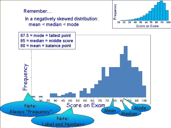
Remember… In a negatively skewed distribution: mean < median < mode Frequency 87. 5 = mode = tallest point 85 = median = middle score 80 = mean = balance point Note: Always “frequency” Score on Exam Note: Label and Numbers Mean Mode Median

Schedule of readings Before our fourth exam (April 30 th) Lind Chapter 13: Linear Regression and Correlation Chapter 14: Multiple Regression Chapter 15: Chi-Square Plous Chapter 17: Social Influences Chapter 18: Group Judgments and Decisions

Over next couple of lectures 4/16/15 Logic of hypothesis testing with Correlations Interpreting the Correlations and scatterplots Simple and Multiple Regression Using correlation for predictions r versus r 2 Regression uses the predictor variable (independent) to make predictions about the predicted variable (dependent) Coefficient of correlation is name for “r” Coefficient of determination is name for “r 2” (remember it is always positive – no direction info) Standard error of the estimate is our measure of the variability of the dots around the regression line (average deviation of each data point from the regression line – like standard deviation) Coefficient of regression will “b” for each variable (like slope)

Homework due – Tuesday (April 21 st) On class website: Please print and complete homeworksheet #16 Interpreting Correlation and Simple Regression

Correlation: Measure of how two variables co-occur and also can be used for prediction • Range between -1 and +1 • The closer to zero the weaker the relationship and the worse the prediction • Positive or negative Remember, We’ll call the correlations “r” Revisit this slide

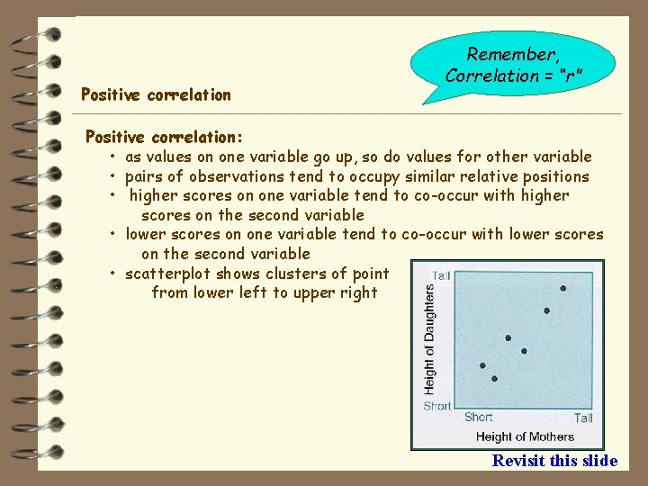
Positive correlation Remember, Correlation = “r” Positive correlation: • as values on one variable go up, so do values for other variable • pairs of observations tend to occupy similar relative positions • higher scores on one variable tend to co-occur with higher scores on the second variable • lower scores on one variable tend to co-occur with lower scores on the second variable • scatterplot shows clusters of point from lower left to upper right Revisit this slide

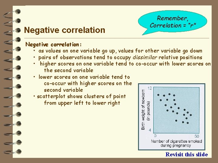
Negative correlation Remember, Correlation = “r” Negative correlation: • as values on one variable go up, values for other variable go down • pairs of observations tend to occupy dissimilar relative positions • higher scores on one variable tend to co-occur with lower scores on the second variable • lower scores on one variable tend to co-occur with higher scores on the second variable • scatterplot shows clusters of point from upper left to lower right Revisit this slide

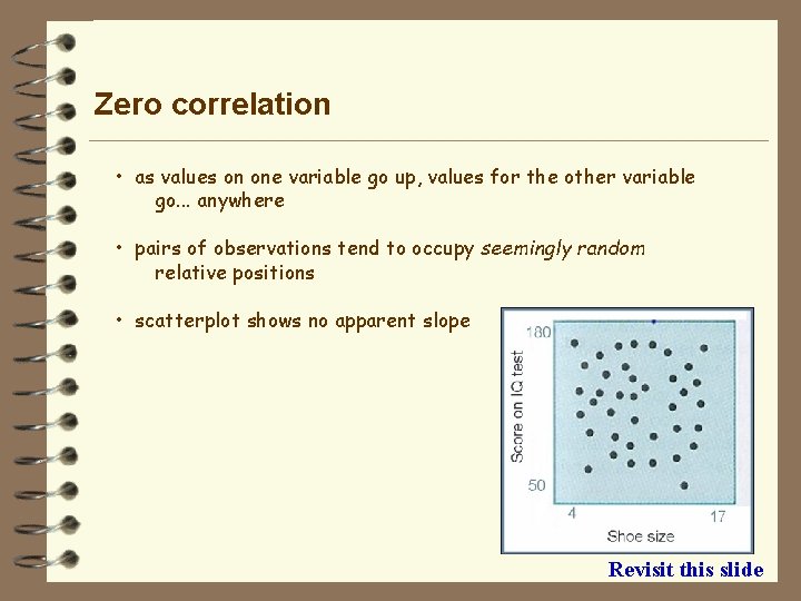
Zero correlation • as values on one variable go up, values for the other variable go. . . anywhere • pairs of observations tend to occupy seemingly random relative positions • scatterplot shows no apparent slope Revisit this slide

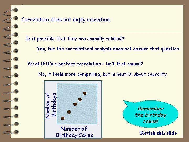
Correlation does not imply causation Is it possible that they are causally related? Yes, but the correlational analysis does not answer that question What if it’s a perfect correlation – isn’t that causal? Number of Birthdays No, it feels more compelling, but is neutral about causality Number of Birthday Cakes Remember the birthday cakes! Revisit this slide

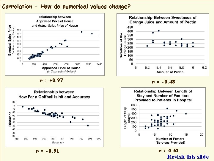
Correlation - How do numerical values change? r = +0. 97 r = -0. 91 r = -0. 48 r = 0. 61 Revisit this slide

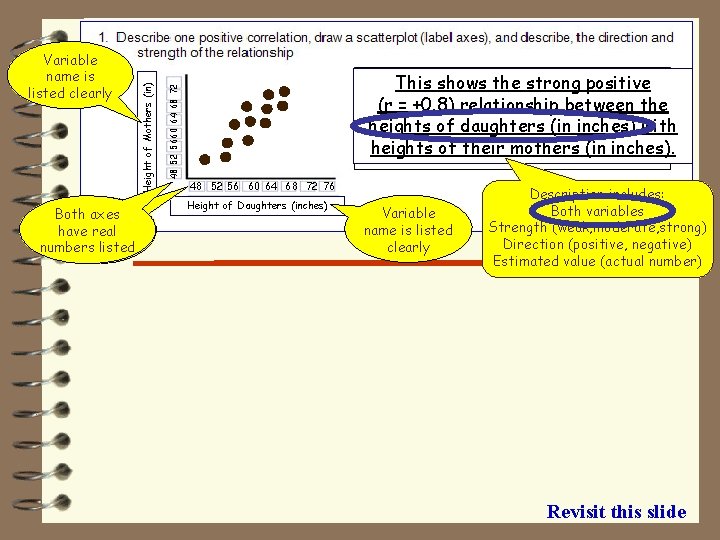
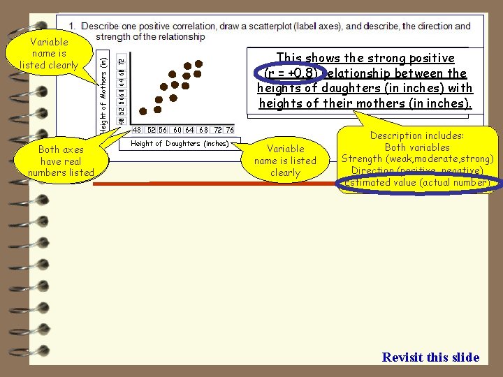
Bothaxes have real and values numbers listed are labeled 48 52 5660 64 68 72 Height of Mothers (in) Variable name is listed clearly This shows the strong positive (r = +0. 8) relationship between the heights of daughters (in inches) with heights of their mothers (in inches). 48 52 56 60 64 68 72 76 Height of Daughters (inches) Variable name is listed clearly Description includes: Both variables Strength (weak, moderate, strong) Direction (positive, negative) Estimated value (actual number) Revisit this slide

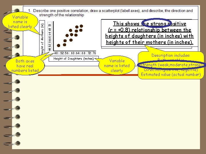
Bothaxes have real and values numbers listed are labeled 48 52 5660 64 68 72 Height of Mothers (in) Variable name is listed clearly This shows the strong positive (r = +0. 8) relationship between the heights of daughters (in inches) with heights of their mothers (in inches). 48 52 56 60 64 68 72 76 Height of Daughters (inches) Variable name is listed clearly Description includes: Both variables Strength (weak, moderate, strong) Direction (positive, negative) Estimated value (actual number)

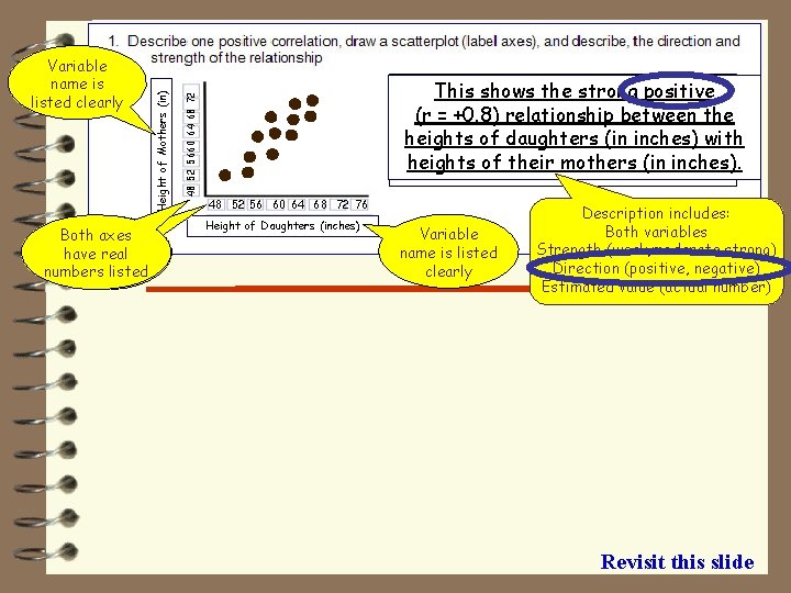
Bothaxes have real and values numbers listed are labeled 48 52 5660 64 68 72 Height of Mothers (in) Variable name is listed clearly This shows the strong positive (r = +0. 8) relationship between the heights of daughters (in inches) with heights of their mothers (in inches). 48 52 56 60 64 68 72 76 Height of Daughters (inches) Variable name is listed clearly Description includes: Both variables Strength (weak, moderate, strong) Direction (positive, negative) Estimated value (actual number) Revisit this slide

Bothaxes have real and values numbers listed are labeled 48 52 5660 64 68 72 Height of Mothers (in) Variable name is listed clearly This shows the strong positive (r = +0. 8) relationship between the heights of daughters (in inches) with heights of their mothers (in inches). 48 52 56 60 64 68 72 76 Height of Daughters (inches) Variable name is listed clearly Description includes: Both variables Strength (weak, moderate, strong) Direction (positive, negative) Estimated value (actual number) Revisit this slide

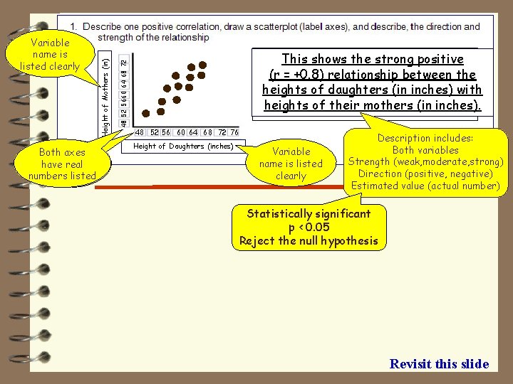
Bothaxes have real and values numbers listed are labeled 48 52 5660 64 68 72 Height of Mothers (in) Variable name is listed clearly This shows the strong positive (r = +0. 8) relationship between the heights of daughters (in inches) with heights of their mothers (in inches). 48 52 56 60 64 68 72 76 Height of Daughters (inches) Variable name is listed clearly Description includes: Both variables Strength (weak, moderate, strong) Direction (positive, negative) Estimated value (actual number) Statistically significant p < 0. 05 Reject the null hypothesis Revisit this slide

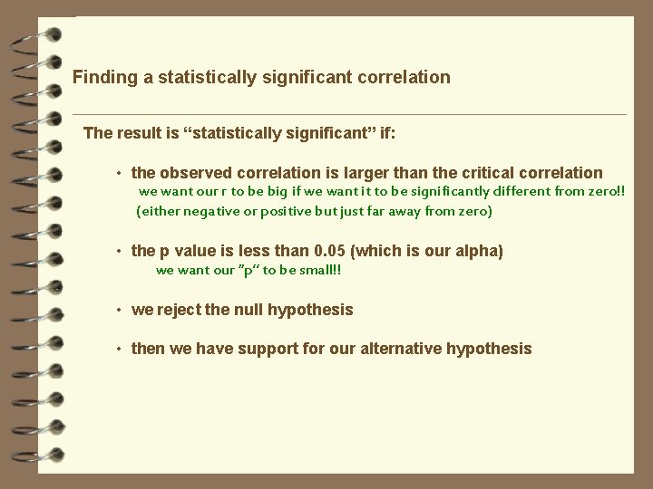
Finding a statistically significant correlation The result is “statistically significant” if: • the observed correlation is larger than the critical correlation we want our r to be big if we want it to be significantly different from zero!! (either negative or positive but just far away from zero) • the p value is less than 0. 05 (which is our alpha) we want our “p” to be small!! • we reject the null hypothesis • then we have support for our alternative hypothesis

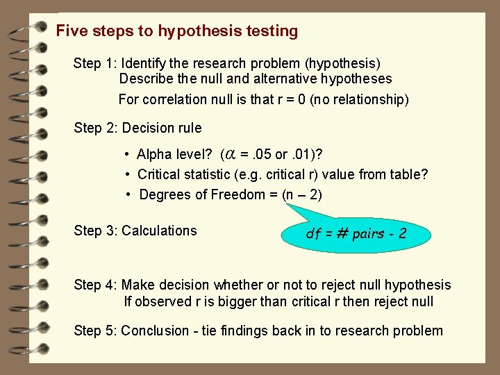
Five steps to hypothesis testing Step 1: Identify the research problem (hypothesis) Describe the null and alternative hypotheses For correlation null is that r = 0 (no relationship) Step 2: Decision rule • Alpha level? (α =. 05 or. 01)? • Critical statistic (e. g. critical r) value from table? • Degrees of Freedom = (n – 2) Step 3: Calculations df = # pairs - 2 Step 4: Make decision whether or not to reject null hypothesis If observed r is bigger than critical r then reject null Step 5: Conclusion - tie findings back in to research problem

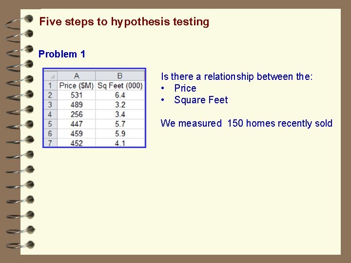
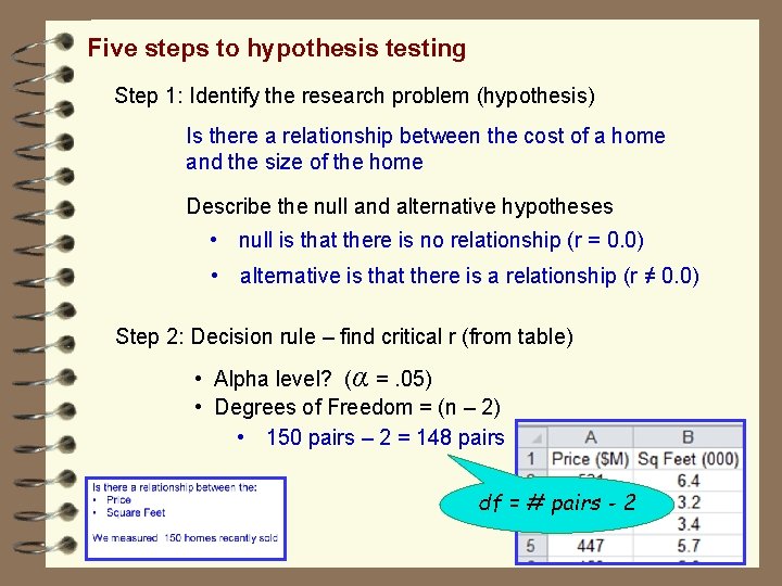
Five steps to hypothesis testing Problem 1 Is there a relationship between the: • Price • Square Feet We measured 150 homes recently sold

Five steps to hypothesis testing Step 1: Identify the research problem (hypothesis) Is there a relationship between the cost of a home and the size of the home Describe the null and alternative hypotheses • null is that there is no relationship (r = 0. 0) • alternative is that there is a relationship (r ≠ 0. 0) Step 2: Decision rule – find critical r (from table) • Alpha level? (α =. 05) • Degrees of Freedom = (n – 2) • 150 pairs – 2 = 148 pairs df = # pairs - 2

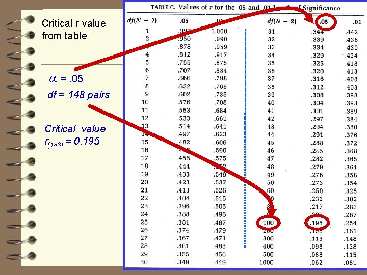
Critical r value from table α =. 05 df = 148 pairs Critical value r(148) = 0. 195 df = # pairs - 2

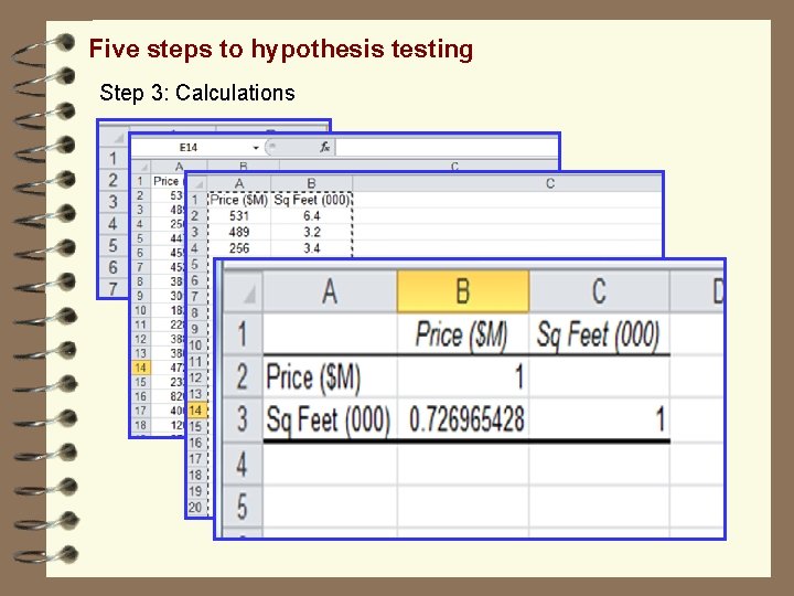
Five steps to hypothesis testing Step 3: Calculations

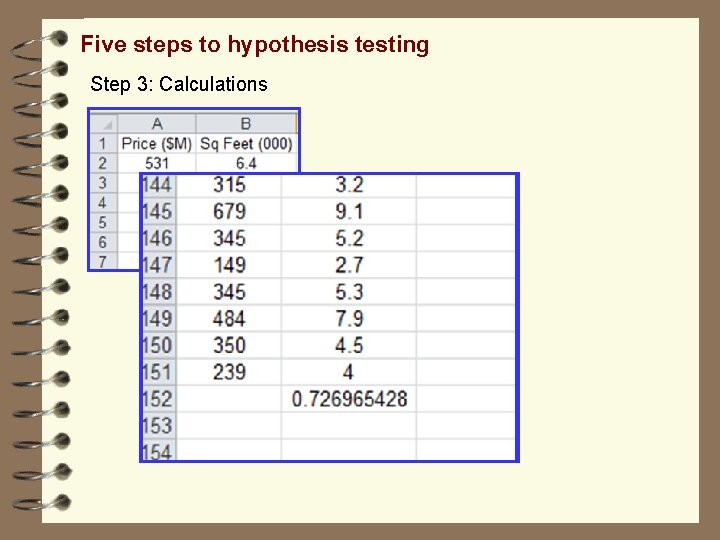
Five steps to hypothesis testing Step 3: Calculations

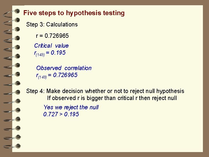
Five steps to hypothesis testing Step 3: Calculations r = 0. 726965 Critical value r(148) = 0. 195 Observed correlation r(148) = 0. 726965 Step 4: Make decision whether or not to reject null hypothesis If observed r is bigger than critical r then reject null Yes we reject the null 0. 727 > 0. 195

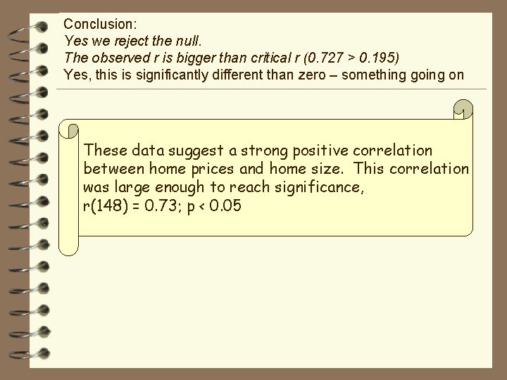
Conclusion: Yes we reject the null. The observed r is bigger than critical r (0. 727 > 0. 195) Yes, this is significantly different than zero – something going on These data suggest a strong positive correlation between home prices and home size. This correlation was large enough to reach significance, r(148) = 0. 73; p < 0. 05

Finding a statistically significant correlation The result is “statistically significant” if: • the observed correlation is larger than the critical correlation we want our r to be big if we want it to be significantly different from zero!! (either negative or positive but just far away from zero) • the p value is less than 0. 05 (which is our alpha) we want our “p” to be small!! • we reject the null hypothesis • then we have support for our alternative hypothesis

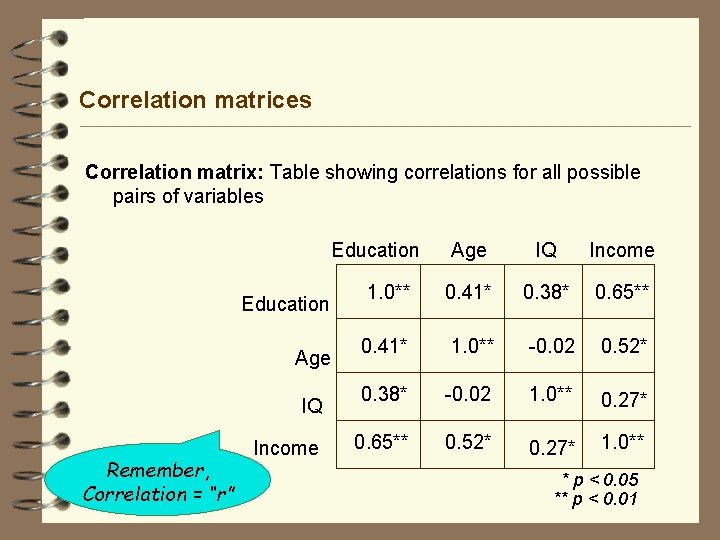
Correlation matrices Correlation matrix: Table showing correlations for all possible pairs of variables Education Age IQ Remember, Correlation = “r” Income Age IQ Income 1. 0** 0. 41* 0. 38* 0. 65** 0. 41* 1. 0** -0. 02 0. 52* 0. 38* -0. 02 1. 0** 0. 27* 0. 65** 0. 52* 0. 27* 1. 0** * p < 0. 05 ** p < 0. 01

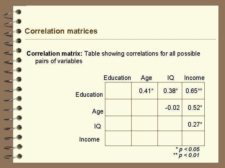
Correlation matrices Correlation matrix: Table showing correlations for all possible pairs of variables Education Age IQ Income 0. 41* 0. 38* 0. 65** -0. 02 0. 52* 0. 27* Income * p < 0. 05 ** p < 0. 01

Finding a statistically significant correlation The result is “statistically significant” if: • the observed correlation is larger than the critical correlation we want our r to be big if we want it to be significantly different from zero!! (either negative or positive but just far away from zero) • the p value is less than 0. 05 (which is our alpha) we want our “p” to be small!! • we reject the null hypothesis • then we have support for our alternative hypothesis

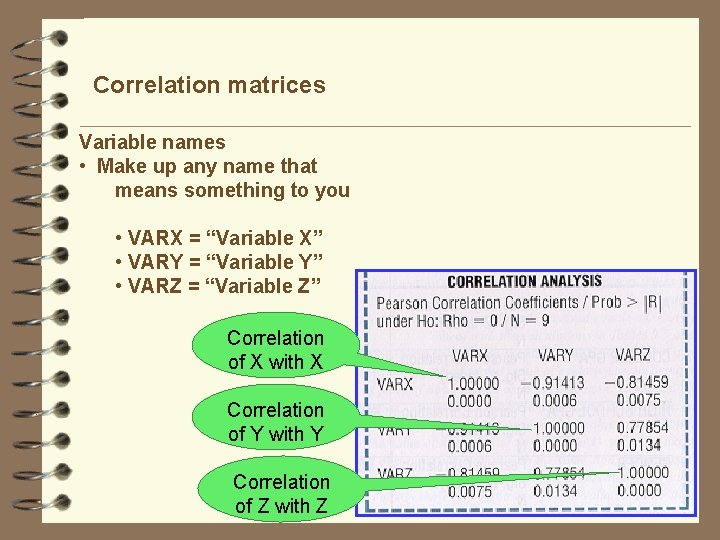
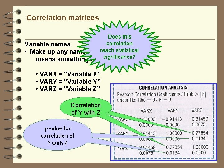
Correlation matrices Variable names • Make up any name that means something to you • VARX = “Variable X” • VARY = “Variable Y” • VARZ = “Variable Z” Correlation of X with X Correlation of Y with Y Correlation of Z with Z

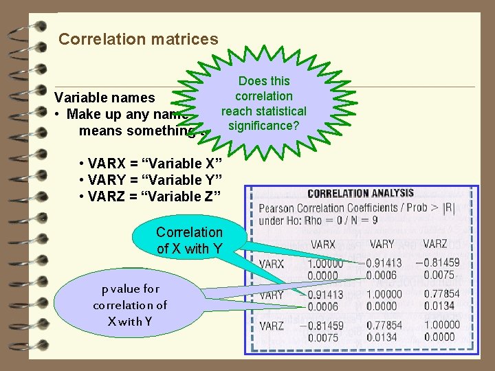
Correlation matrices Does this correlation Variable names • Make up any name that reach statistical significance? means something to you • VARX = “Variable X” • VARY = “Variable Y” • VARZ = “Variable Z” Correlation of X with Y valuefor ppvalue correlation of of with XX with YY

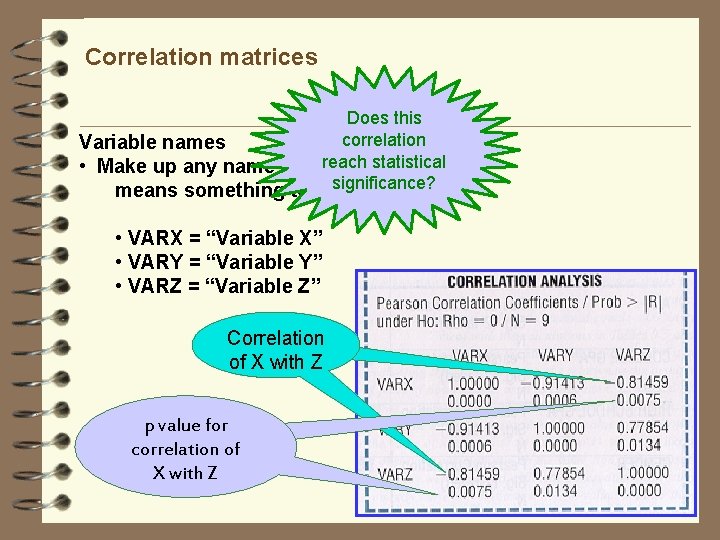
Correlation matrices Does this correlation Variable names • Make up any name that reach statistical significance? means something to you • VARX = “Variable X” • VARY = “Variable Y” • VARZ = “Variable Z” Correlation of X with Z p value for correlationofof. X Xwith. ZZ

Correlation matrices Does this correlation Variable names • Make up any name that reach statistical significance? means something to you • VARX = “Variable X” • VARY = “Variable Y” • VARZ = “Variable Z” Correlation of Y with Z valuefor ppvalue correlationof of correlation with. ZZ YYwith

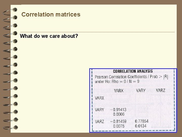
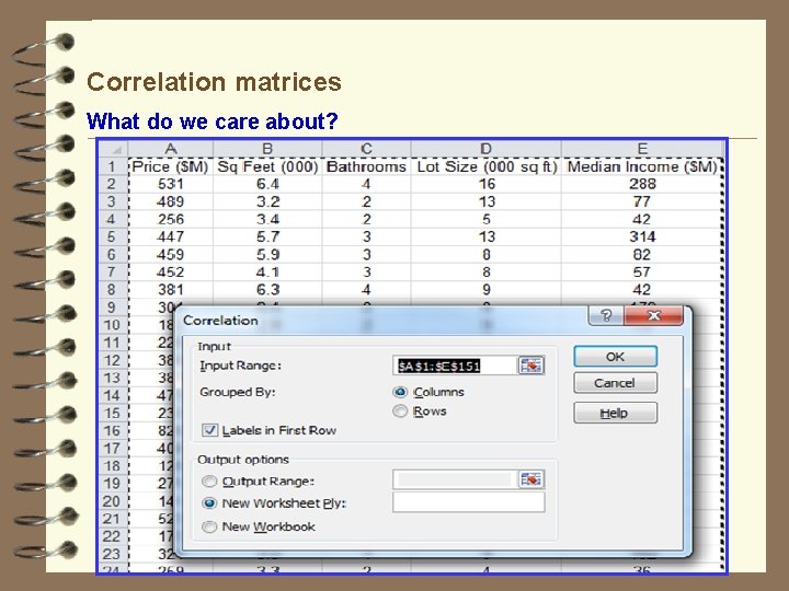
Correlation matrices What do we care about?

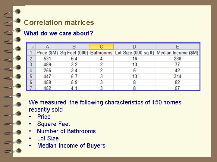
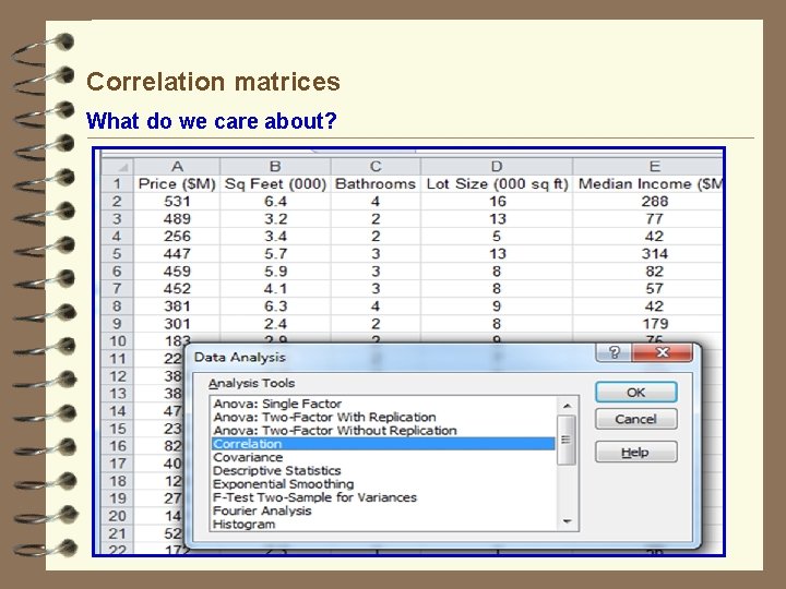
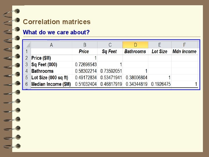
Correlation matrices What do we care about? We measured the following characteristics of 150 homes recently sold • Price • Square Feet • Number of Bathrooms • Lot Size • Median Income of Buyers

Correlation matrices What do we care about?

Correlation matrices What do we care about?

Correlation matrices What do we care about?

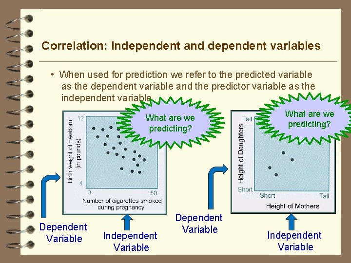
Correlation: Independent and dependent variables • When used for prediction we refer to the predicted variable as the dependent variable and the predictor variable as the independent variable What are we predicting? Dependent Variable Independent Variable Dependent Variable What are we predicting? Independent Variable

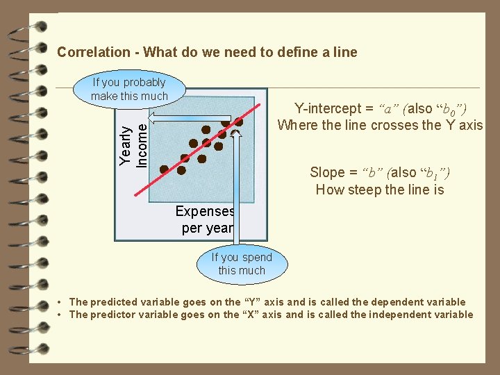
Correlation - What do we need to define a line If you probably make this much Yearly Income Y-intercept = “a” (also “b 0”) Where the line crosses the Y axis Slope = “b” (also “b 1”) How steep the line is Expenses per year If you spend this much • The predicted variable goes on the “Y” axis and is called the dependent variable • The predictor variable goes on the “X” axis and is called the independent variable

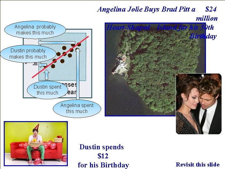
Angelina Jolie Buys Brad Pitt a $24 million Heart-Shaped Island for his 50 th Birthday Yearly Income Angelina probably makes this much Dustin probably makes this much Expenses Dustin spent per year this much Angelina spent this much Dustin spends $12 for his Birthday Revisit this slide

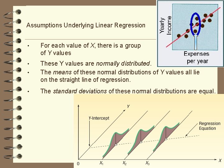
Assumptions Underlying Linear Regression • For each value of X, there is a group of Y values • • These Y values are normally distributed. The means of these normal distributions of Y values all lie on the straight line of regression. • The standard deviations of these normal distributions are equal.

Correlation - the prediction line - what is it good for? Prediction line • makes the relationship easier to see (even if specific observations - dots - are removed) • identifies the center of the cluster of (paired) observations • identifies the central tendency of the relationship (kind of like a mean) • can be used for prediction • should be drawn to provide a “best fit” for the data • should be drawn to provide maximum predictive power for the data • should be drawn to provide minimum predictive error

Correlation: Independent and dependent variables • When used for prediction we refer to the predicted variable as the dependent variable and the predictor variable as the independent variable What are we predicting? Dependent Variable Independent Variable Dependent Variable What are we predicting? Independent Variable

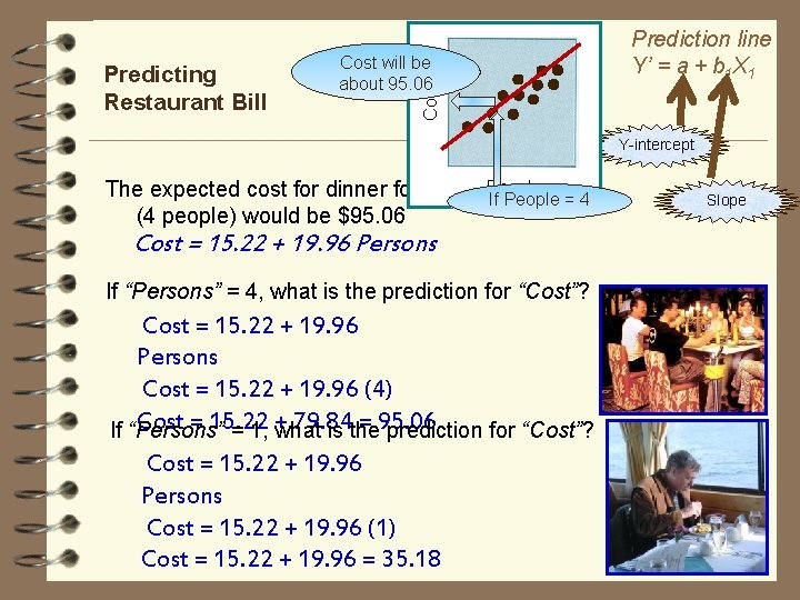
Cost will be about 95. 06 Cost Predicting Restaurant Bill Prediction line Y’ = a + b 1 X 1 Y-intercept People The expected cost for dinner for two couples If People = 4 (4 people) would be $95. 06 Cost = 15. 22 + 19. 96 Persons If “Persons” = 4, what is the prediction for “Cost”? Cost = 15. 22 + 19. 96 Persons Cost = 15. 22 + 19. 96 (4) Cost = 15. 22 79. 84 = 95. 06 If “Persons” = 1, + what is the prediction for “Cost”? Cost = 15. 22 + 19. 96 Persons Cost = 15. 22 + 19. 96 (1) Cost = 15. 22 + 19. 96 = 35. 18 Slope

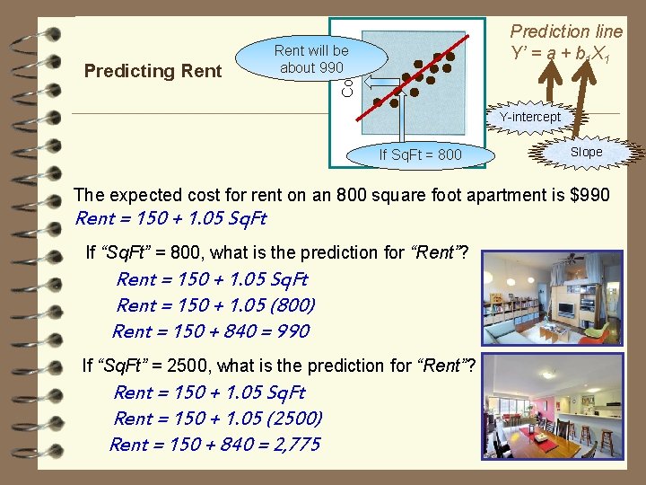
Rent will be about 990 Cost Predicting Rent Prediction line Y’ = a + b 1 X 1 Y-intercept Square If Sq. Ft. Feet = 800 Slope The expected cost for rent on an 800 square foot apartment is $990 Rent = 150 + 1. 05 Sq. Ft If “Sq. Ft” = 800, what is the prediction for “Rent”? Rent = 150 + 1. 05 Sq. Ft Rent = 150 + 1. 05 (800) Rent = 150 + 840 = 990 If “Sq. Ft” = 2500, what is the prediction for “Rent”? Rent = 150 + 1. 05 Sq. Ft Rent = 150 + 1. 05 (2500) Rent = 150 + 840 = 2, 775