Roo Stats Cms a tool for analyses modelling

Roo. Stats. Cms: a tool for analyses modelling, combination and statistical studies D. Piparo, G. Schott, G. Quast Institut für Experimentelle Kernphysik Universität Karlsruhe

Outline • The need for a tool • Roo. Stats. Cms (RSC) • A Roo. Fit interlude • The three parts – Modelling • The datacard • Inspect your model – Statistical studies and limits • Profile Likelihood • Hypothesis separation and “modified frequentist approach” – Exclusion – Plotting classes 19. 11. 08 D. Piparo 2

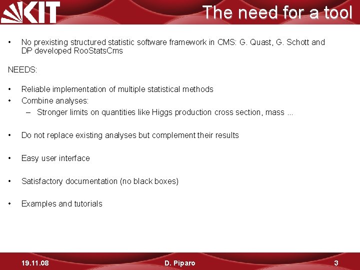
The need for a tool • No prexisting structured statistic software framework in CMS: G. Quast, G. Schott and DP developed Roo. Stats. Cms NEEDS: • • Reliable implementation of multiple statistical methods Combine analyses: – Stronger limits on quantities like Higgs production cross section, mass. . . • Do not replace existing analyses but complement their results • Easy user interface • Satisfactory documentation (no black boxes) • Examples and tutorials 19. 11. 08 D. Piparo 3

Roo. Stats. Cms • • • Originally thought for the CMS Higgs Working Group and a CMS (EKP) exclusive product Based on Roo. Fit (Part of the ROOT distribution) Three parts: – Modelling and combination – Statistical methods – Advanced graphic routines It comes with CINT dictionaries (macros, interactive root). Available to CMS and EKP at: www-ekp. physik. uni-karlsruhe. de/~Roo. Stats. Cms – – • Visit our wiki for username and password Statistical methods and graphic routines public: www-ekp. physik. uni-karlsruhe. de/~Roo. Stats. Karlsruhe Big effort for documentation: 1. RSC website and Doxygen of every class, method and member 2. Wikipages with links to RSC presentations (~15) and workshop • • 3. https: //twiki. cern. ch/twiki/bin/view/CMS/Higgs. WGRoo. Stats. Cms http: //www-ekp. physik. uni-karlsruhe. de/~twiki/bin/view/Ekp. Cms/Roo. Stats. Cms An internal CMS note in preparation 19. 11. 08 D. Piparo 4

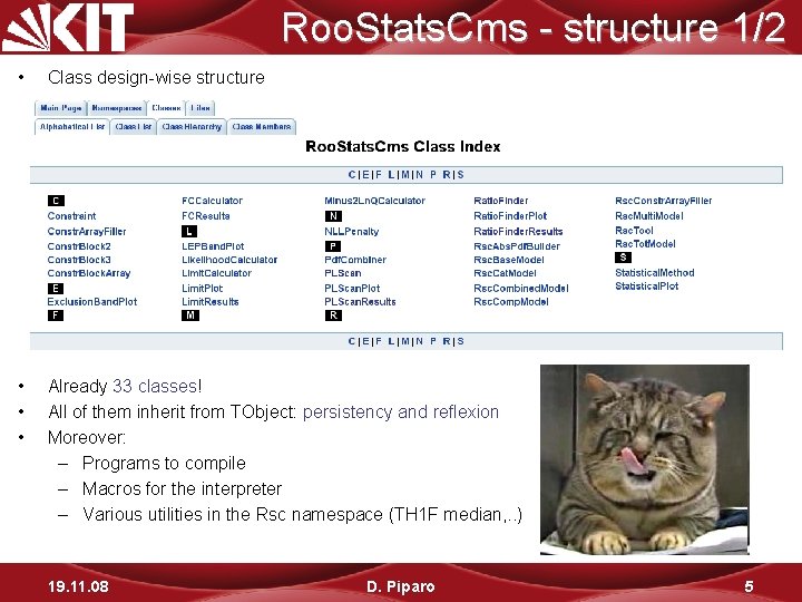
Roo. Stats. Cms - structure 1/2 • Class design-wise structure • • • Already 33 classes! All of them inherit from TObject: persistency and reflexion Moreover: – Programs to compile – Macros for the interpreter – Various utilities in the Rsc namespace (TH 1 F median, . . ) 19. 11. 08 D. Piparo 5

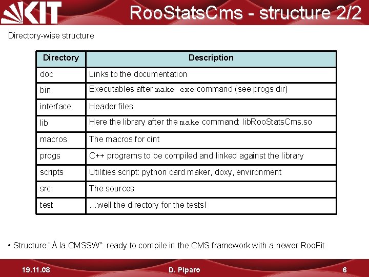
Roo. Stats. Cms - structure 2/2 Directory-wise structure Directory Description doc Links to the documentation bin Executables after make exe command (see progs dir) interface Header files lib Here the library after the make command: lib. Roo. Stats. Cms. so macros The macros for cint progs C++ programs to be compiled and linked against the library scripts Utilities script: python card maker, doxy, environment src The sources test …well the directory for the tests! • Structure “À la CMSSW”: ready to compile in the CMS framework with a newer Roo. Fit 19. 11. 08 D. Piparo 6

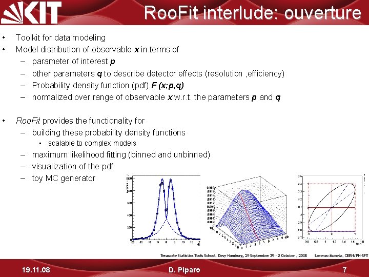
Roo. Fit interlude: ouverture • • Toolkit for data modeling Model distribution of observable x in terms of – parameter of interest p – other parameters q to describe detector effects (resolution , efficiency) – Probability density function (pdf) F (x; p, q) – normalized over range of observable x w. r. t. the parameters p and q • Roo. Fit provides the functionality for – building these probability density functions • scalable to complex models – maximum likelihood fitting (binned and unbinned) – visualization of the pdf – toy MC generator 19. 11. 08 D. Piparo 7

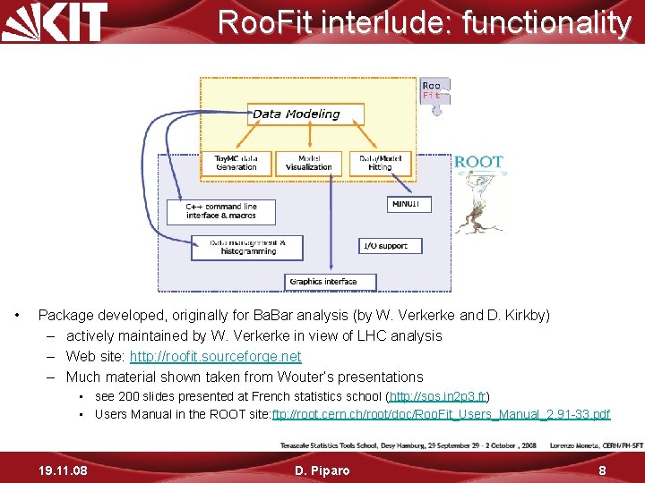
Roo. Fit interlude: functionality • Package developed, originally for Ba. Bar analysis (by W. Verkerke and D. Kirkby) – actively maintained by W. Verkerke in view of LHC analysis – Web site: http: //roofit. sourceforge. net – Much material shown taken from Wouter’s presentations • see 200 slides presented at French statistics school (http: //sos. in 2 p 3. fr) • Users Manual in the ROOT site: ftp: //root. cern. ch/root/doc/Roo. Fit_Users_Manual_2. 91 -33. pdf 19. 11. 08 D. Piparo 8

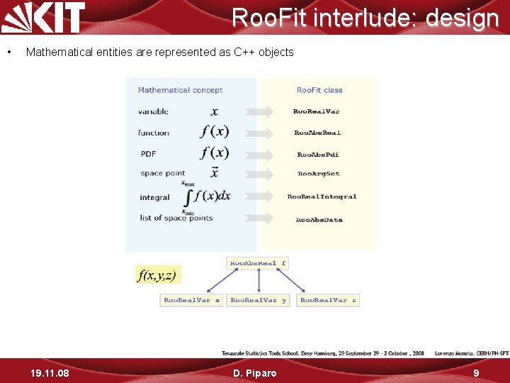
Roo. Fit interlude: design • Mathematical entities are represented as C++ objects 19. 11. 08 D. Piparo 9

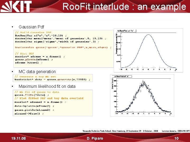
Roo. Fit interlude : an example • Gaussian Pdf • MC data generation • Maximum likelihood fit on data 19. 11. 08 D. Piparo 10

RSC: A solid tool • RSC is in “production phase”: – Around since the beginning of the year 2008 – Workshop at CERN in June – Approved results: http: //cms-physics. web. cern. ch/cms-physics/public/HIG-08 -008 -pas. pdf – Coming soon results: HIG-008 -06 HWW – CMS statistics committee blessed the tool (internal note in preparation) • Grégory in permanent contact with them – Interest of other working groups – Negotiations for integration in CMS Software framework (CMSSW) – Base of a common tool with Atlas • Work in progress: firsts commits in ROOT are taking place – New manpower: Mario Pelliccioni (former Ba. Bar) from Universita’ di Torino • Made in EKP (Quast, Schott, Piparo): – Personal assistance at 8 th floor! 19. 11. 08 D. Piparo 11

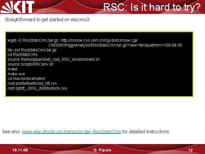
RSC: Is it hard to try? Straightforward to get started on ekpcms 3: wget -O Roo. Stats. Cms. tar. gz http: //cmssw. cvs. cern. ch/cgi-bin/cmssw. cgi/ CMSSW/Higgs. Analysis/Roo. Stats. Cms. tar. gz? view=tar&pathrev=V 00 -04 -00 tar -zxf Roo. Stats. Cms. tar. gz cd Roo. Stats. Cms source /home/piparo/set_root_RSC_environment. sh source scripts/RSCenv. sh make exe cd macros/examples/ root profilelikelihood_htt. cxx root qqhtt_-2 ln. Q_distributions. cxx See also: www-ekp. physik. uni-karlsruhe. de/~Roo. Stats. Cms for detailed instructions 19. 11. 08 D. Piparo 12

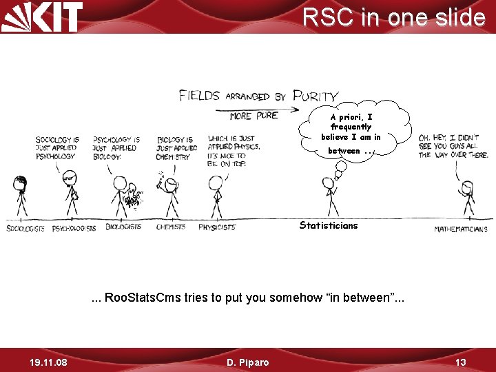
RSC in one slide A priori, I frequently believe I am in between. . . Statisticians . . . Roo. Stats. Cms tries to put you somehow “in between”. . . 19. 11. 08 D. Piparo 13

The Three Parts • Analyses modeling and combination • Statistical Methods and limits • Graphics routines 19. 11. 08 D. Piparo 14

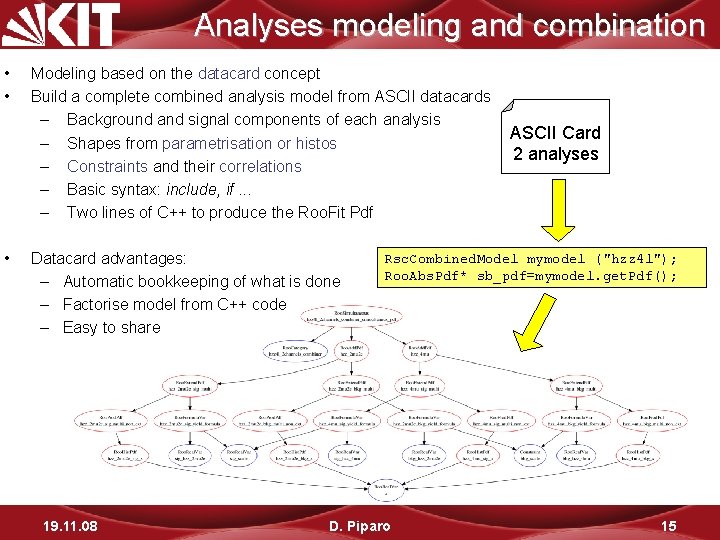
Analyses modeling and combination • • • Modeling based on the datacard concept Build a complete combined analysis model from ASCII datacards – Background and signal components of each analysis – Shapes from parametrisation or histos – Constraints and their correlations – Basic syntax: include, if. . . – Two lines of C++ to produce the Roo. Fit Pdf Datacard advantages: – Automatic bookkeeping of what is done – Factorise model from C++ code – Easy to share 19. 11. 08 ASCII Card 2 analyses Rsc. Combined. Model mymodel ("hzz 4 l"); Roo. Abs. Pdf* sb_pdf=mymodel. get. Pdf(); D. Piparo 15

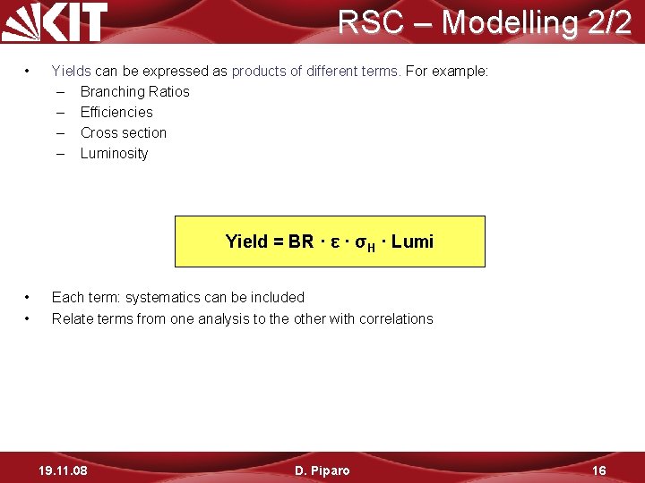
RSC – Modelling 2/2 • Yields can be expressed as products of different terms. For example: – Branching Ratios – Efficiencies – Cross section – Luminosity Yield = BR · ε · σH · Lumi • • Each term: systematics can be included Relate terms from one analysis to the other with correlations 19. 11. 08 D. Piparo 16

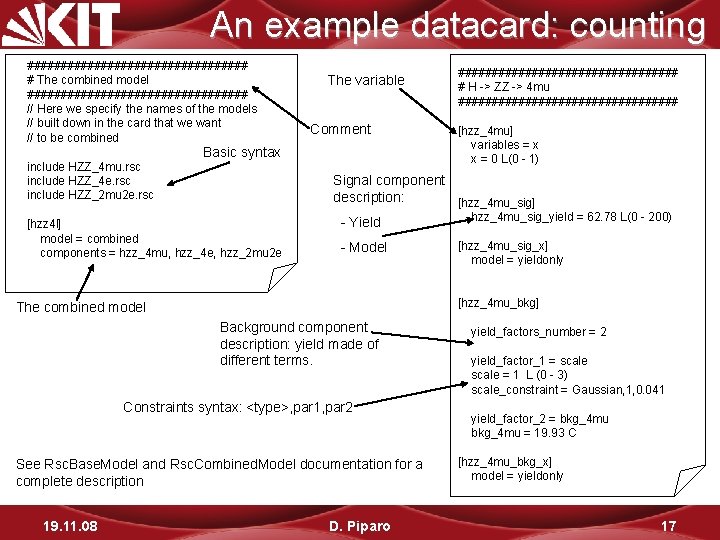
An example datacard: counting ################# # The combined model ################# // Here we specify the names of the models // built down in the card that we want // to be combined include HZZ_4 mu. rsc include HZZ_4 e. rsc include HZZ_2 mu 2 e. rsc The variable Comment Basic syntax [hzz 4 l] model = combined components = hzz_4 mu, hzz_4 e, hzz_2 mu 2 e [hzz_4 mu] variables = x x = 0 L(0 - 1) Signal component description: [hzz_4 mu_sig] hzz_4 mu_sig_yield = 62. 78 L(0 - 200) - Yield - Model [hzz_4 mu_sig_x] model = yieldonly [hzz_4 mu_bkg] The combined model Background component description: yield made of different terms. Constraints syntax: <type>, par 1, par 2 See Rsc. Base. Model and Rsc. Combined. Model documentation for a complete description 19. 11. 08 ################# # H -> ZZ -> 4 mu ################# D. Piparo yield_factors_number = 2 yield_factor_1 = scale = 1 L (0 - 3) scale_constraint = Gaussian, 1, 0. 041 yield_factor_2 = bkg_4 mu = 19. 93 C [hzz_4 mu_bkg_x] model = yieldonly 17

An example datacard: shapes [hgg_cat 0] variables = mh mh = 115 L(90 - 180) // [Ge. V/c^{2}] [hgg_cat 0_sig] yield_factors_number = 3 yield_factor_1 = lumi = 1 C yield_factor_2 = n_events_hgg_115_cat 0_sig n_events_hgg_cat 0_sig = 3. 9577 yield_factor_3 = scale_sig = 1 L (0 - 5) [hgg_cat 0_sig_mh] model = four. Gaussians hgg_115_cat 0_sig_mh_mean 1 = 114. 654 +/- 0. 107106 C hgg_115_cat 0_sig_mh_mean 2 = 115. 146 +/- 2. 37687 C hgg_115_cat 0_sig_mh_mean 3 = 114. 12 +/- 0. 581539 C hgg_115_cat 0_sig_mh_mean 4 = 109. 979 +/- 11. 036 C hgg_115_cat 0_sig_mh_sigma 1 = 0. 6075 +/- 0. 0888951 C hgg_115_cat 0_sig_mh_sigma 2 = 0. 601995 +/- 129. 141 C hgg_115_cat 0_sig_mh_sigma 3 = 2. 1119 +/- 0. 526549 C hgg_115_cat 0_sig_mh_sigma 4 = 8. 16619 +/- 7. 75118 C hgg_115_cat 0_sig_mh_frac 1 = 0. 999893 +/- 0. 500053 C hgg_115_cat 0_sig_mh_frac 2 = 0. 762761 +/- 0. 0870296 C hgg_115_cat 0_sig_mh_frac 3 = 0. 98815 +/- 0. 0207781 C // The combined model of HZZ and Hgg include hzz_combined. rsc Include hgg_12_categories. rsc [hgg_hzz_combined] model = combined components = hzz, hgg_cat 0, hgg_cat 1, . . . , hgg_cat 11 19. 11. 08 Multiple components [hgg_cat 0_bkg] number_components = 2 yield_factors_number = 3 yield_factor_1 = lumi = 1 C yield_factor_2 = n_events_hgg_115_cat 0_bkg n_events_hgg_cat 0_bkg = 988. 389 yield_factor_3 = scale_bkg = 1 L (0 - 5) [hgg_cat 0_bkg 1] qqhtt_bkg 1_yield = 1 C [hgg_cat 0_bkg 2] qqhtt_bkg 2_yield = 1. 35 C Histogram and parametric models mixed [hgg_cat 0_bkg 1_mh] model = double. Gaussian hgg_cat 0_bkg_mh_mean 1 = 52. 3484 +/- 14. 1593 C hgg_cat 0_bkg_mh_mean 2 = 158. 962 +/- 3. 21153 C hgg_cat 0_bkg_mh_sigma 1 = 27. 1791 +/- 2. 37455 C hgg_cat 0_bkg_mh_sigma 2 = 74. 9328 +/- 70. 6298 C hgg_cat 0_bkg_mh_frac = 0. 924937 +/- 0. 0347411 C [hgg_cat 0_bkg 2_mh] model = histo hgg_cat 0_bkg 2_mh _file. Name = htt_inputs. root hgg_cat 0_bkg 2_mh name = background Comment 1. Combination of combined models 2. Counting combined with shape analyses D. Piparo 18

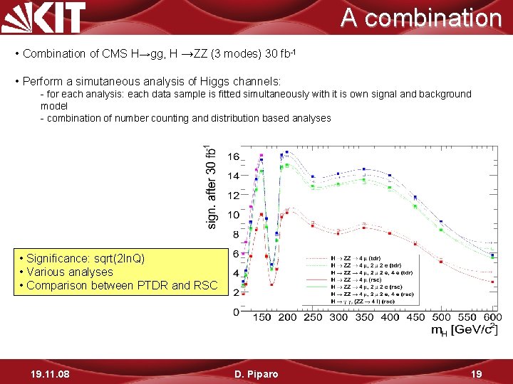
A combination • Combination of CMS H→gg, H →ZZ (3 modes) 30 fb-1 • Perform a simutaneous analysis of Higgs channels: - for each analysis: each data sample is fitted simultaneously with it is own signal and background model - combination of number counting and distribution based analyses • Significance: sqrt(2 ln. Q) • Various analyses • Comparison between PTDR and RSC 19. 11. 08 D. Piparo 19

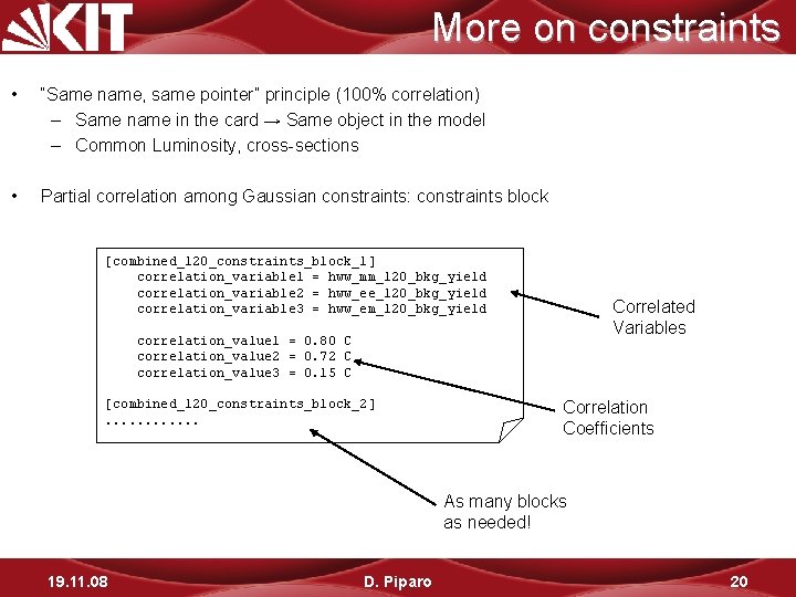
More on constraints • “Same name, same pointer” principle (100% correlation) – Same name in the card → Same object in the model – Common Luminosity, cross-sections • Partial correlation among Gaussian constraints: constraints block [combined_120_constraints_block_1] correlation_variable 1 = hww_mm_120_bkg_yield correlation_variable 2 = hww_ee_120_bkg_yield correlation_variable 3 = hww_em_120_bkg_yield Correlated Variables correlation_value 1 = 0. 80 C correlation_value 2 = 0. 72 C correlation_value 3 = 0. 15 C [combined_120_constraints_block_2]. . . Correlation Coefficients As many blocks as needed! 19. 11. 08 D. Piparo 20

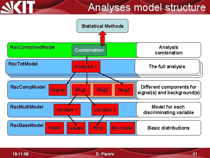
Analyses model structure Statistical Methods Rsc. Combined. Model Rsc. Tot. Model Rsc. Comp. Model Rsc. Multi. Model Rsc. Base. Model 19. 11. 08 Analysis combination Combination Analysis 11 Signal Bkg 1 Variable 1 Histo Gauss The full analysis Thefullanalysis Bkg 2 Bkg 3 Variable 2 Poly My model D. Piparo Different components for signal(s) and background(s) Model for each discriminating variable Basic distributions 21

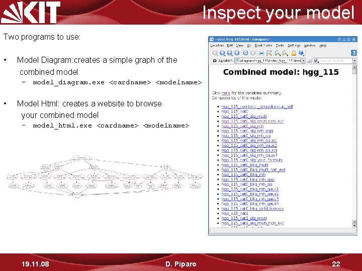
Inspect your model Two programs to use: • Model Diagram: creates a simple graph of the combined model – model_diagram. exe <cardname> <modelname> • Model Html: creates a website to browse your combined model – model_html. exe <cardname> <modelname> 19. 11. 08 D. Piparo 22

The Three Parts • Analyses modeling and combination • Statistical Methods and limits • Graphics routines 19. 11. 08 D. Piparo 23

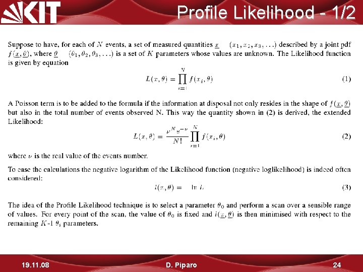
Profile Likelihood - 1/2 19. 11. 08 D. Piparo 24

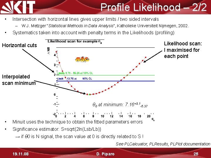
Profile Likelihood – 2/2 • Intersection with horizontal lines gives upper limits / two sided intervals – W. J. Metzger “Statistical Methods in Data Analysis”, Katholieke Universiteit Nijmegen, 2002. • Systematics taken into account with penalty terms in the Likelihoods (profiling) Likelihood scan: l maximised for each point Horizontal cuts Interpolated scan minimum θ 0 at minimum: 7. 16+8. 1 -5. 37 • Minuit uses the technique to obtain the fitted parameters errors • Significance estimator: S=sqrt(2 ln(Lsb/Lb)) → if θ 0 is N signal, the scan value at 0 is directly related to S ! See PLCalcuator, PLResults, PLPlot documentation 19. 11. 08 D. Piparo 25

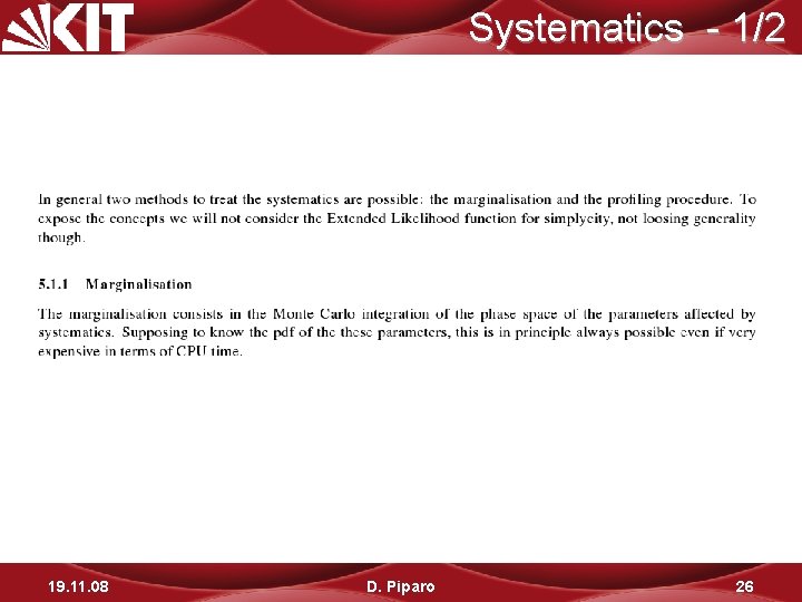
Systematics - 1/2 19. 11. 08 D. Piparo 26

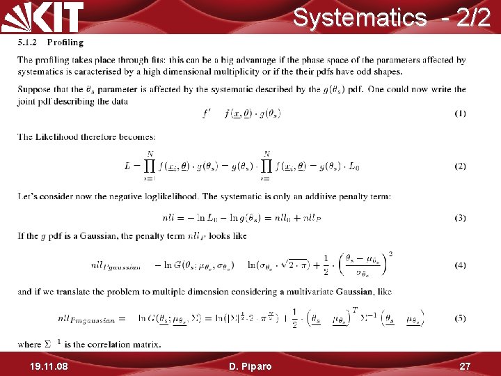
Systematics - 2/2 19. 11. 08 D. Piparo 27

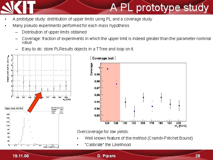
A PL prototype study • A prototype study: distribution of upper limits using PL and a coverage study • Many pseudo experiments performed for each mass hypothesis – Distribution of upper limits obtained – Coverage: fraction of experiments in which the upper limit is indeed greater than the parameter nominal value – Easy to do: store PLResults objects in a TTree and loop on it. Overcoverage for low yields: 19. 11. 08 • Well known feature of the method (Cramér-Fréchet Bound) • “Calibrate” the Likelihood D. Piparo 28

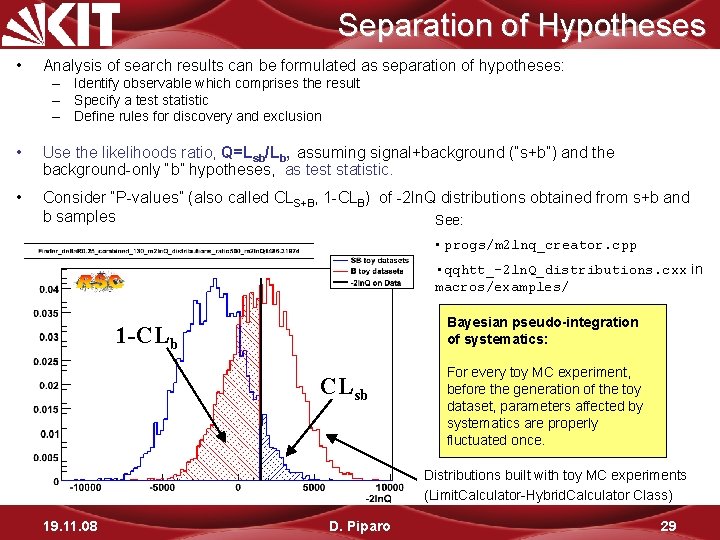
Separation of Hypotheses • Analysis of search results can be formulated as separation of hypotheses: – Identify observable which comprises the result – Specify a test statistic – Define rules for discovery and exclusion • Use the likelihoods ratio, Q=Lsb/Lb, assuming signal+background (“s+b”) and the background-only “b” hypotheses, as test statistic. • Consider “P-values” (also called CLS+B, 1 -CLB) of -2 ln. Q distributions obtained from s+b and b samples See: • progs/m 2 lnq_creator. cpp • qqhtt_-2 ln. Q_distributions. cxx in macros/examples/ Bayesian pseudo-integration of systematics: 1 -CLb CLsb For every toy MC experiment, before the generation of the toy dataset, parameters affected by systematics are properly fluctuated once. Distributions built with toy MC experiments (Limit. Calculator-Hybrid. Calculator Class) 19. 11. 08 D. Piparo 29

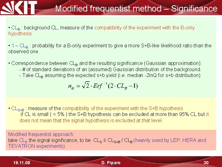
Modified frequentist method – Significance • CLB : background CL, measure of the compatibility of the experiment with the B-only hypothesis • 1 – CLB : probability for a B-only experiment to give a more S+B-likelihood ratio than the observed one • Correspondence between CLB and the resulting significance (Gaussian approximation): - # of standard deviations of an (assumed) Gaussian distribution of the background. - Take CLB assuming the expected s+b yield (i. e. median -2 ln. Q for s+b distribution) • CLS+B : measure of the compatibility of the experiment with the S+B hypothesis if CL is small ( < 5% ) the S+B hypothesis can be excluded at more than 95% CL but it does not mean that the signal hypothesis is excluded at that level Modified frequentist approach: take CLS the signal significance, to be: CLS ≡ CLS+B / CLB (heavily used by LEP, HERA and TEVATRON experiments) 19. 11. 08 D. Piparo 30

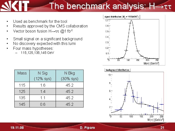
The benchmark analysis: H→ • • • Used as benchmark for the tool Results approved by the CMS collaboration Vector boson fusion H→ @1 fb-1 • • • Small signal on a significant background No discovery expected with this lumi Four mass hypotheses: – 115, 125, 135, 145 Ge. V Mass N Sig (12% sys) N Bkg (30% sys) 115 1. 6 45. 2 125 1. 4 45. 2 135 1. 1 45. 2 145 0. 6 45. 2 19. 11. 08 D. Piparo 31

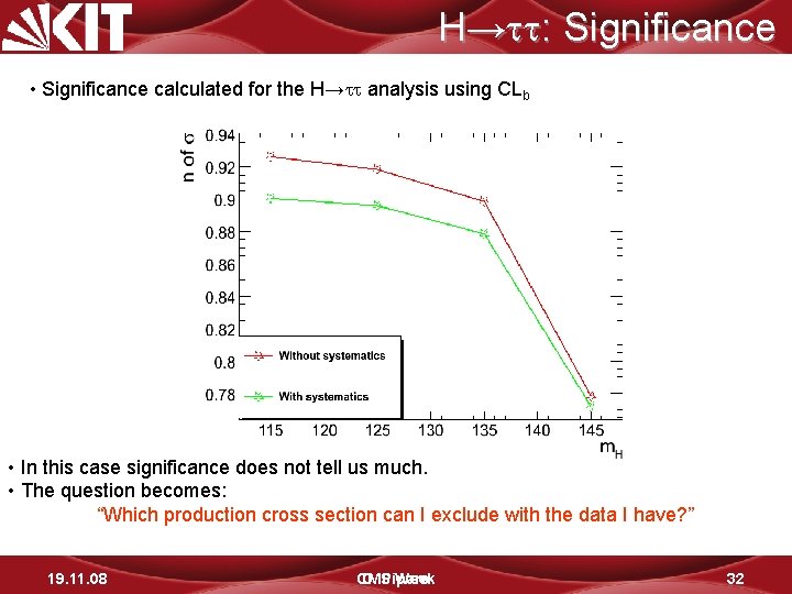
H→ : Significance • Significance calculated for the H→ analysis using CLb • In this case significance does not tell us much. • The question becomes: “Which production cross section can I exclude with the data I have? ” 19. 11. 08 CMS D. Piparo Week 32

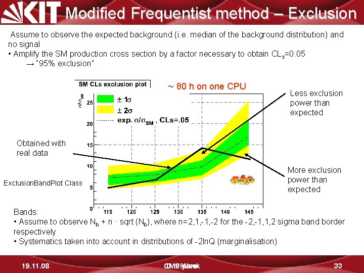
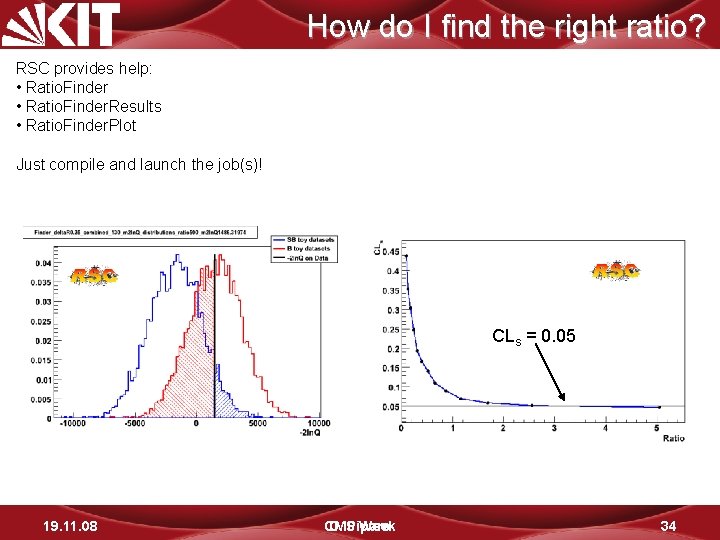
Modified Frequentist method – Exclusion Assume to observe the expected background (i. e. median of the background distribution) and no signal • Amplify the SM production cross section by a factor necessary to obtain CLs=0. 05 → “ 95% exclusion” ~ 80 h on one CPU Less exclusion power than expected Obtained with real data More exclusion power than expected Exclusion. Band. Plot Class Bands: • Assume to observe Nb + n · sqrt (Nb), where n=2, 1, -2 for the -2, -1, 1, 2 sigma band border respectively • Systematics taken into account in distributions of -2 ln. Q (marginalisation) 19. 11. 08 CMS D. Piparo Week 33

How do I find the right ratio? RSC provides help: • Ratio. Finder. Results • Ratio. Finder. Plot Just compile and launch the job(s)! CLs = 0. 05 19. 11. 08 CMS D. Piparo Week 34

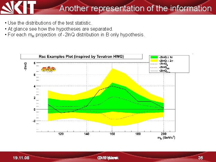
Another representation of the information • Use the distributions of the test statistic. • At glance see how the hypotheses are separated. • For each m. H projection of -2 ln. Q distribution in B only hypothesis. 19. 11. 08 CMS D. Piparo Week 35

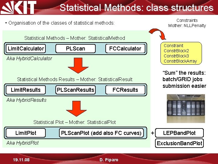
Statistical Methods: class structures Constraints Mother: NLLPenalty • Organisation of the classes of statistical methods: Statistical Methods – Mother: Statistical. Method Limit. Calculator PLScan Constraint Constr. Block 2 Constr. Block 3 Constr. Block. Array FCCalculator Aka Hybrid. Calculator “Sum” the results: batch/GRID jobs submission easier Statistical Methods Results – Mother: Statistical. Result Limit. Results Limit. Calculator PLScan. Results FCResults Aka Hybrid. Results Statistical Plot – Mother: Statistical. Plot Limit. Plot PLScan. Plot (add also FC curves) LEPBand. Plot Exclusion. Band. Plot Aka Hybrid. Plot 19. 11. 08 + D. Piparo

The Three Parts • Analyses modeling and combination • Statistical Methods and limits • Graphics routines 19. 11. 08 D. Piparo 37

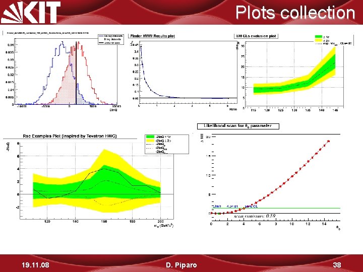
Plots collection 19. 11. 08 D. Piparo 38

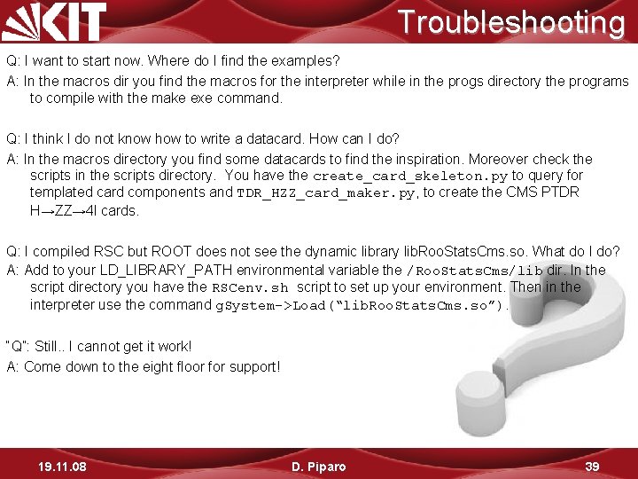
Troubleshooting Q: I want to start now. Where do I find the examples? A: In the macros dir you find the macros for the interpreter while in the progs directory the programs to compile with the make exe command. Q: I think I do not know how to write a datacard. How can I do? A: In the macros directory you find some datacards to find the inspiration. Moreover check the scripts in the scripts directory. You have the create_card_skeleton. py to query for templated card components and TDR_HZZ_card_maker. py, to create the CMS PTDR H→ZZ→ 4 l cards. Q: I compiled RSC but ROOT does not see the dynamic library lib. Roo. Stats. Cms. so. What do I do? A: Add to your LD_LIBRARY_PATH environmental variable the /Roo. Stats. Cms/lib dir. In the script directory you have the RSCenv. sh script to set up your environment. Then in the interpreter use the command g. System->Load(“lib. Roo. Stats. Cms. so”). “Q”: Still. . I cannot get it work! A: Come down to the eight floor for support! 19. 11. 08 D. Piparo 39

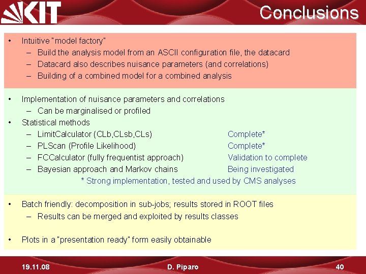
Conclusions • Intuitive “model factory” – Build the analysis model from an ASCII configuration file, the datacard – Datacard also describes nuisance parameters (and correlations) – Building of a combined model for a combined analysis • Implementation of nuisance parameters and correlations – Can be marginalised or profiled Statistical methods – Limit. Calculator (CLb, CLs) Complete* – PLScan (Profile Likelihood) Complete* – FCCalculator (fully frequentist approach) Validation to complete – Bayesian approach and Markov chains Being investigated * Strong implementation, tested and used by CMS analyses • • Batch friendly: decomposition in sub-jobs; results stored in ROOT files – Results can be merged and exploited by results classes • Plots in a “presentation ready” form easily obtainable 19. 11. 08 D. Piparo 40