Stats 346 3 Stats 848 3 Multivariate Data

Stats 346. 3 Stats 848. 3 Multivariate Data Analysis

Instructor: W. H. Laverty Office: 235 Mc. Lean Hall Phone: 966 -6096 Lectures: MWF 12: 30 am - 1: 20 pm Arts 104 Evaluation: Assignments, Term tests - 40% Final Examination - 60%

Dates for midterm tests: 1. Friday, February 08 2. Friday, March 22 Each test and the Final Exam are Open Book Students are allowed to take in Notes, texts, formula sheets, calculators (laptop computers. )

Text: Stat 346 –Multivariate Statistical Methods – Donald Morrison Not Required - I will give a list of other useful texts that will be in the library

Bibliography 1. Cooley, W. W. , and Lohnes P. R. (1962). Multivariate Procedures for the Behavioural Sciences, Wiley, New York. 2. Fienberg, S. (1980), Analysis of Cross-Classified Data , MIT Press, Cambridge, Mass. 3. Fingelton, B. (1984), Models for Category Counts , Cambridge University Press. 4. Johnson, R. A. and Wichern D. W. Applied Multivariate Statistical Analysis , Prentice Hall. 5. Morrison, D. F. (1976), Multivariate Statistical Methods , Mc. Graw-Hill, New York. 6. Seal, H. (1968), Multivariate Statistical Analysis for Biologists , Metheun, London 7. Alan Agresti (1990) Categorical Data Analysis, Wiley, New York.

• The lectures will be given in Power Point • They are now posted on the Stats 346 web page

Course Outline

Introduction

Review of Linear Algebra and Matrix Analysis Chapter 2 Review of Linear Statistical Theory Chapter 1

Multivariate Normal distribution • Multivariate Data plots • Correlation - sample estimates and tests • Canonical Correlation Chapter 3

Mean Vectors and Covariance matrices • Single sample procedures • Two sample procedures • Profile Analysis Chapter 4

Multivariate Analysis of Variance (MANOVA) Chapter 5

Classification and Discrimination • Discriminant Analysis • Logistic Regression (if time permits) • Cluster Analysis Chapters 6

The structure of correlation • Principal Components Analysis (PCA) • Factor Analysis Chapter 9

Multivariate Multiple Regression (if time permits) References TBA

Discrete Multivariate Analysis (if time permits) References: TBA

Introduction

Multivariate Data • • • We have collected data for each case in the sample or population on not just one variable but on several variables – X 1, X 2, … Xp This is likely the situation – very rarely do you collect data on a single variable. The variables maybe 1. Discrete (Categorical) 2. Continuous (Numerical) • The variables may be 1. Dependent (Response variables) 2. Independent (Predictor variables)

A chart illustrating Statistical Procedures Independent variables Dependent Variables Categorical Continuous Categorical Multiway frequency Analysis (Log Linear Model) Discriminant Analysis Continuous ANOVA (single dep var) MANOVA (Mult dep var) Continuous & Categorical ? ? MULTIPLE REGRESSION (single dep variable) MULTIVARIATE MULTIPLE REGRESSION (multiple dependent variable) ? ? Continuous & Categorical Discriminant Analysis ANACOVA (single dep var) MANACOVA (Mult dep var) ? ?

Multivariate Techniques can be classified as follows: 1. Techniques that are direct analogues of univariate procedures. • • • There are univariate techniques that are then generalized to the multivariate situarion e. g. The two independent sample t test, generalized to Hotelling’s T 2 test ANOVA (Analysis of Variance) generalized to MANOVA (Multivariate Analysis of Variance)

2. Techniques that are purely multivariate procedures. • • Correlation, Partial correlation, Multiple correlation, Canonical Correlation Principle component Analysis, Factor Analysis - These are techniques for studying complicated correlation structure amongst a collection of variables

3. Techniques for which a univariate procedures could exist but these techniques become much more interesting in the multivariate setting. • Cluster Analysis and Classification - • Here we try to identify subpopulations from the data Discriminant Analysis - In Discriminant Analysis, we attempt to use a collection of variables to identify the unknown population for which a case is a member

An Example: A survey was given to 132 students • Male=35, • Female=97 They rated, on a Likert scale • 1 to 5 • their agreement with each of 40 statements. All statements are related to the Meaning of Life

Questions and Statements

Statements - continued

Cluster Analysis of n = 132 university students using responses from Meaning of Life questionnaire (40 questions)

Discriminant Analysis of n = 132 university students into the three identified populations

A Review of Linear Algebra With some Additions

Matrix Algebra Definition An n × m matrix, A, is a rectangular array of elements n = # of columns m = # of rows dimensions = n × m

Definition A vector, v, of dimension n is an n × 1 matrix rectangular array of elements vectors will be column vectors (they may also be row vectors)

A vector, v, of dimension n can be thought a point in n dimensional space

v 3 v 2 v 1

Matrix Operations Addition Let A = (aij) and B = (bij) denote two n × m matrices Then the sum, A + B, is the matrix The dimensions of A and B are required to be both n × m.

Scalar Multiplication Let A = (aij) denote an n × m matrix and let c be any scalar. Then c. A is the matrix

Addition for vectors v 3 v 2 v 1

Scalar Multiplication for vectors v 3 v 2 v 1

Matrix multiplication Let A = (aij) denote an n × m matrix and B = (bjl) denote an m × k matrix Then the n × k matrix C = (cil) where is called the product of A and B and is denoted by A∙B

In the case that A = (aij) is an n × m matrix and B = v = (vj) is an m × 1 vector Then w = A∙v = (wi) where is an n × 1 vector w 3 v 3 w 2 v 1 w 1

Definition An n × n identity matrix, I, is the square matrix Note: 1. AI = A 2. IA = A.

Definition (The inverse of an n × n matrix) Let A denote the n × n matrix Let B denote an n × n matrix such that AB = BA = I, If the matrix B exists then A is called invertible Also B is called the inverse of A and is denoted by A-1

The Woodbury Theorem where the inverses

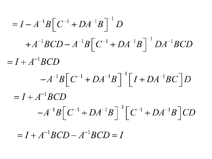
Proof: Let Then all we need to show is that H(A + BCD) = (A + BCD) H = I.

The Woodbury theorem can be used to find the inverse of some pattern matrices: Example: Find the inverse of the n × n matrix

where hence and

Thus Now using the Woodbury theorem

Thus

where

Note: for n = 2

Also

Now

and This verifies that we have calculated the inverse

Block Matrices Let the n × m matrix be partitioned into sub-matrices A 11, A 12, A 21, A 22, Similarly partition the m × k matrix

Product of Blocked Matrices Then

The Inverse of Blocked Matrices Let the n × n matrix be partitioned into sub-matrices A 11, A 12, A 21, A 22, Similarly partition the n × n matrix Suppose that B = A-1

Product of Blocked Matrices Then

Hence From (1) From (3)

Hence or using the Woodbury Theorem Similarly

From and similarly

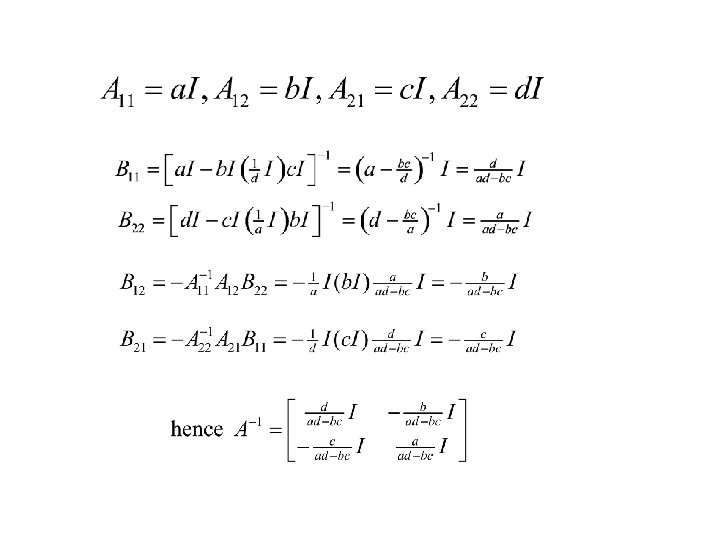
Summarizing Let Suppose that A-1 = B then

Example Let Find A-1 = B

The transpose of a matrix Consider the n × m matrix, A then the m × n matrix, (also denoted by AT) is called the transpose of A

Symmetric Matrices • An n × n matrix, A, is said to be symmetric if Note:

The trace and the determinant of a square matrix Let A denote then n × n matrix Then

also where

Some properties

Some additional Linear Algebra

Inner product of vectors Let denote two p × 1 vectors. Then.

Note: Let denote two p × 1 vectors. Then.

Note: Let denote two p × 1 vectors. Then. 0

Special Types of Matrices 1. Orthogonal matrices – A matrix is orthogonal if P'P = PP' = I – In this cases P-1=P'. – Also the rows (columns) of P have length 1 and are orthogonal to each other

Suppose P is an orthogonal matrix then Let denote p × 1 vectors. Orthogonal transformation preserve length and angles – Rotations about the origin, Reflections

Example The following matrix P is orthogonal

Special Types of Matrices (continued) 2. Positive definite matrices – A symmetric matrix, A, is called positive definite if: – A symmetric matrix, A, is called positive semi definite if:

If the matrix A is positive definite then

Theorem The matrix A is positive definite if

Special Types of Matrices (continued) 3. Idempotent matrices – A symmetric matrix, E, is called idempotent if: – Idempotent matrices project vectors onto a linear subspace

Definition Let A be an n × n matrix Let then l is called an eigenvalue of A and is called an eigenvector of A and

Note:

= polynomial of degree n in l. Hence there are n possible eigenvalues l 1, … , ln

Thereom If the matrix A is symmetric then the eigenvalues of A, l 1, … , ln, are real. Thereom If the matrix A is positive definite then the eigenvalues of A, l 1, … , ln, are positive. Proof A is positive definite if Let be an eigenvalue and corresponding eigenvector of A.

Thereom If the matrix A is symmetric and the eigenvalues of A are l 1, … , ln, with corresponding eigenvectors If li ≠ lj then Proof: Note

Thereom If the matrix A is symmetric with distinct eigenvalues, l 1, … , ln, with corresponding eigenvectors Assume

proof Note and P is called an orthogonal matrix

therefore thus

Comment The previous result is also true if the eigenvalues are not distinct. Namely if the matrix A is symmetric with eigenvalues, l 1, … , ln, with corresponding eigenvectors of unit length

An algorithm for computing eigenvectors, eigenvalues of positive definite matrices • Generally to compute eigenvalues of a matrix we need to first solve the equation for all values of l. – |A – l. I| = 0 (a polynomial of degree n in l) • Then solve the equation for the eigenvector

Recall that if A is positive definite then It can be shown that and that

Thus for large values of m The algorithim 1. Compute powers of A - A 2 , A 4 , A 8 , A 16 , . . . 2. Rescale (so that largest element is 1 (say)) 3. Continue until there is no change, The resulting matrix will be 4. Find 5. Find

To find 6. Repeat steps 1 to 5 with the above matrix to find 7. Continue to find

Example A=

Differentiation with respect to a vector, matrix

Differentiation with respect to a vector Let denote a p × 1 vector. Let function of the components of. denote a

Rules 1. Suppose

2. Suppose

Example 1. Determine when is a maximum or minimum. solution

2. Determine when is a maximum if Assume A is a positive definite matrix. solution l is the Lagrange multiplier. This shows that is an eigenvector of A. Thus is the eigenvector of A associated with the largest eigenvalue, l.

Differentiation with respect to a matrix Let X denote a q × p matrix. Let f (X) denote a function of the components of X then:

Example Let X denote a p × p matrix. Let f (X) = ln |X| Solution Note Xij are cofactors = (i, j)th element of X-1

Example Let X and A denote p × p matrices. Let f (X) = tr (AX) Solution

Differentiation of a matrix of functions Let U = (uij) denote a q × p matrix of functions of x then:

Rules:

Proof:

Proof:

Proof:

The Generalized Inverse of a matrix

Recall B (denoted by A-1) is called the inverse of A if AB = BA = I • A-1 does not exist for all matrices A • A-1 exists only if A is a square matrix and |A| ≠ 0 • If A-1 exists then the system of linear equations has a unique solution

Definition B (denoted by A-) is called the generalized inverse (Moore – Penrose inverse) of A if 1. ABA = A 2. BAB = B 3. (AB)' = AB 4. (BA)' = BA Note: A- is unique Proof: Let B 1 and B 2 satisfying 1. ABi. A = A 2. Bi. ABi = Bi 3. (ABi)' = ABi 4. (Bi. A)' = Bi. A

Hence B 1 = B 1 AB 2 AB 1 = B 1 (AB 2)'(AB 1) ' = B 1 B 2'A'B 1'A'= B 1 B 2'A' = B 1 AB 2 AB 2 = (B 1 A)(B 2 A)B 2 = (B 1 A)'(B 2 A)'B 2 = A'B 1'A'B 2 = A'B 2= (B 2 A)'B 2 = B 2 AB 2 = B 2 The general solution of a system of Equations The general solution where is arbitrary

Suppose a solution exists Let

Calculation of the Moore-Penrose g-inverse Let A be a p×q matrix of rank q < p, Proof thus also

Let B be a p×q matrix of rank p < q, Proof thus also

Let C be a p×q matrix of rank k < min(p, q), then C = AB where A is a p×k matrix of rank k and B is a k×q matrix of rank k Proof is symmetric, as well as

References 1. Matrix Algebra Useful for Statistics, Shayle R. Searle 2. Mathematical Tools for Applied Multivariate Analysis, J. Douglas Carroll, Paul E. Green