Introduction to Roo Fit 1 Introduction and overview

Introduction to Roo. Fit 1. Introduction and overview 2. Creation and basic use of models 3. Composing models 4. Working with (profile) likelihood 5. Simultaneous fits and combined models W. Verkerke (NIKHEF)

1 Introduction & Overview

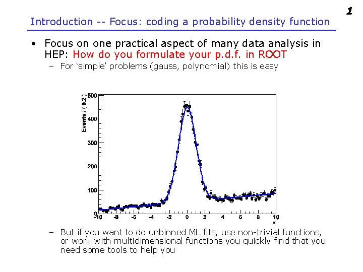
Introduction -- Focus: coding a probability density function • Focus on one practical aspect of many data analysis in HEP: How do you formulate your p. d. f. in ROOT – For ‘simple’ problems (gauss, polynomial) this is easy – But if you want to do unbinned ML fits, use non-trivial functions, or work with multidimensional functions you quickly find that you need some tools to help you 1

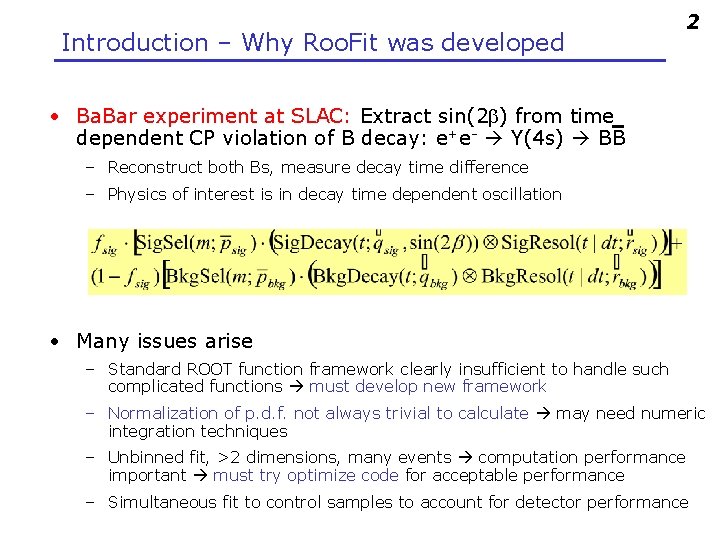
Introduction – Why Roo. Fit was developed 2 • Ba. Bar experiment at SLAC: Extract sin(2 b) from time dependent CP violation of B decay: e+e- Y(4 s) BB – Reconstruct both Bs, measure decay time difference – Physics of interest is in decay time dependent oscillation • Many issues arise – Standard ROOT function framework clearly insufficient to handle such complicated functions must develop new framework – Normalization of p. d. f. not always trivial to calculate may need numeric integration techniques – Unbinned fit, >2 dimensions, many events computation performance important must try optimize code for acceptable performance – Simultaneous fit to control samples to account for detector performance

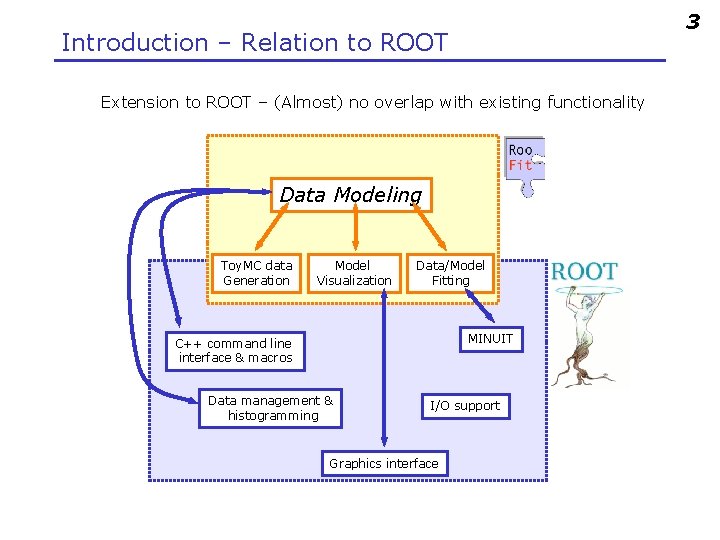
3 Introduction – Relation to ROOT Extension to ROOT – (Almost) no overlap with existing functionality Data Modeling Toy. MC data Generation Model Visualization Data/Model Fitting MINUIT C++ command line interface & macros Data management & histogramming I/O support Graphics interface

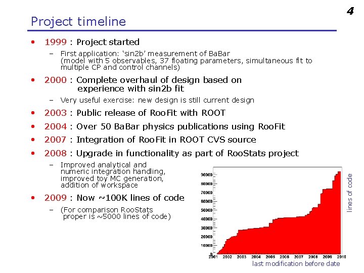
4 Project timeline • 1999 : Project started – First application: ‘sin 2 b’ measurement of Ba. Bar (model with 5 observables, 37 floating parameters, simultaneous fit to multiple CP and control channels) • 2000 : Complete overhaul of design based on experience with sin 2 b fit – Very useful exercise: new design is still current design • 2003 : Public release of Roo. Fit with ROOT • 2004 : Over 50 Ba. Bar physics publications using Roo. Fit • 2007 : Integration of Roo. Fit in ROOT CVS source • 2008 : Upgrade in functionality as part of Roo. Stats project lines of code – Improved analytical and numeric integration handling, improved toy MC generation, addition of workspace • 2009 : Now ~100 K lines of code – (For comparison Roo. Stats proper is ~5000 lines of code) last modification before date

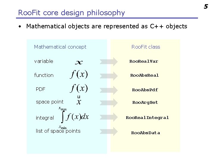
5 Roo. Fit core design philosophy • Mathematical objects are represented as C++ objects Mathematical concept Roo. Fit class variable Roo. Real. Var function Roo. Abs. Real PDF Roo. Abs. Pdf space point Roo. Arg. Set integral list of space points Roo. Real. Integral Roo. Abs. Data

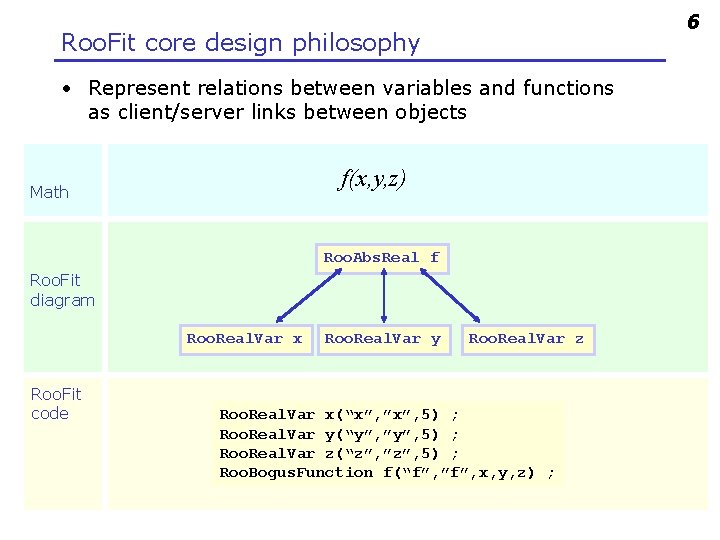
6 Roo. Fit core design philosophy • Represent relations between variables and functions as client/server links between objects f(x, y, z) Math Roo. Abs. Real f Roo. Fit diagram Roo. Real. Var x Roo. Fit code Roo. Real. Var y Roo. Real. Var z Roo. Real. Var x(“x”, ”x”, 5) ; Roo. Real. Var y(“y”, ”y”, 5) ; Roo. Real. Var z(“z”, ”z”, 5) ; Roo. Bogus. Function f(“f”, ”f”, x, y, z) ;

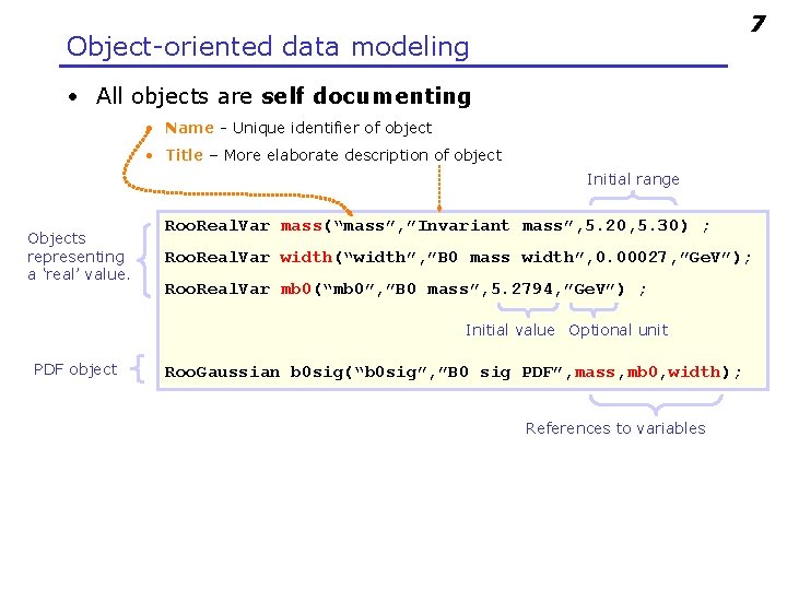
7 Object-oriented data modeling • All objects are self documenting • Name - Unique identifier of object • Title – More elaborate description of object Initial range Objects representing a ‘real’ value. Roo. Real. Var mass(“mass”, ”Invariant mass”, 5. 20, 5. 30) ; Roo. Real. Var width(“width”, ”B 0 mass width”, 0. 00027, ”Ge. V”); Roo. Real. Var mb 0(“mb 0”, ”B 0 mass”, 5. 2794, ”Ge. V”) ; Initial value Optional unit PDF object Roo. Gaussian b 0 sig(“b 0 sig”, ”B 0 sig PDF”, mass, mb 0, width); References to variables

2 Basic use

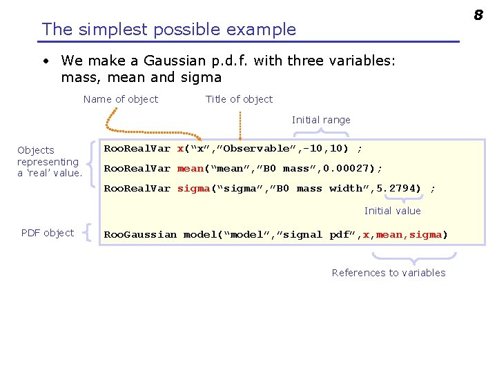
8 The simplest possible example • We make a Gaussian p. d. f. with three variables: mass, mean and sigma Name of object Title of object Initial range Objects representing a ‘real’ value. Roo. Real. Var x(“x”, ”Observable”, -10, 10) ; Roo. Real. Var mean(“mean”, ”B 0 mass”, 0. 00027); Roo. Real. Var sigma(“sigma”, ”B 0 mass width”, 5. 2794) ; Initial value PDF object Roo. Gaussian model(“model”, ”signal pdf”, x, mean, sigma) References to variables

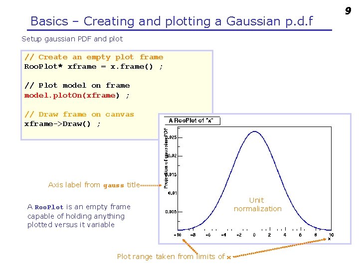
Basics – Creating and plotting a Gaussian p. d. f Setup gaussian PDF and plot // Create an empty plot frame Roo. Plot* xframe = x. frame() ; // Plot model on frame model. plot. On(xframe) ; // Draw frame on canvas xframe->Draw() ; Axis label from gauss title A Roo. Plot is an empty frame capable of holding anything plotted versus it variable Plot range taken from limits of x Unit normalization 9

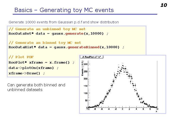
Basics – Generating toy MC events Generate 10000 events from Gaussian p. d. f and show distribution // Generate an unbinned toy MC set Roo. Data. Set* data = gauss. generate(x, 10000) ; // Generate an binned toy MC set Roo. Data. Hist* data = gauss. generate. Binned(x, 10000) ; // Plot PDF Roo. Plot* xframe = x. frame() ; data->plot. On(xframe) ; xframe->Draw() ; Can generate both binned and unbinned datasets 10

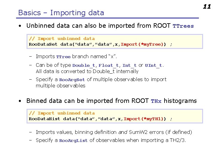
Basics – Importing data • Unbinned data can also be imported from ROOT TTrees // Import unbinned data Roo. Data. Set data(“data”, ”data”, x, Import(*my. Tree)) ; – Imports TTree branch named “x”. – Can be of type Double_t, Float_t, Int_t or UInt_t. All data is converted to Double_t internally – Specify a Roo. Arg. Set of multiple observables to import multiple observables • Binned data can be imported from ROOT THx histograms // Import unbinned data Roo. Data. Hist data(“data”, ”data”, x, Import(*my. TH 1)) ; – Imports values, binning definition and Sum. W 2 errors (if defined) – Specify a Roo. Arg. List of observables when importing a TH 2/3. 11

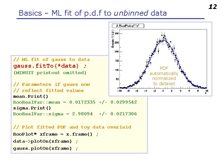
Basics – ML fit of p. d. f to unbinned data // ML fit of gauss to data gauss. fit. To(*data) ; (MINUIT printout omitted) // Parameters if gauss now // reflect fitted values mean. Print() Roo. Real. Var: : mean = 0. 0172335 +/- 0. 0299542 sigma. Print() Roo. Real. Var: : sigma = 2. 98094 +/- 0. 0217306 // Plot fitted PDF and toy data overlaid Roo. Plot* xframe = x. frame() ; data->plot. On(xframe) ; gauss. plot. On(xframe) ; PDF automatically normalized to dataset 12

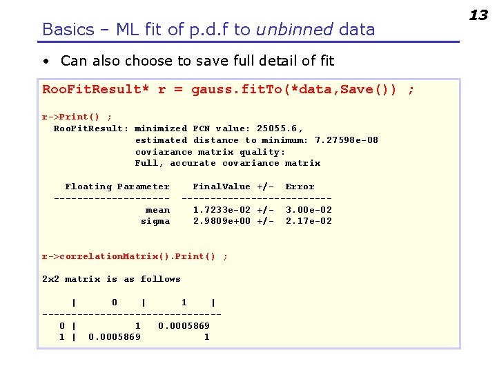
Basics – ML fit of p. d. f to unbinned data • Can also choose to save full detail of fit Roo. Fit. Result* r = gauss. fit. To(*data, Save()) ; r->Print() ; Roo. Fit. Result: minimized FCN value: 25055. 6, estimated distance to minimum: 7. 27598 e-08 coviarance matrix quality: Full, accurate covariance matrix Floating Parameter ----------mean sigma Final. Value +/- Error -------------1. 7233 e-02 +/- 3. 00 e-02 2. 9809 e+00 +/- 2. 17 e-02 r->correlation. Matrix(). Print() ; 2 x 2 matrix is as follows | 0 | 1 | ---------------0 | 1 0. 0005869 1 | 0. 0005869 1 13

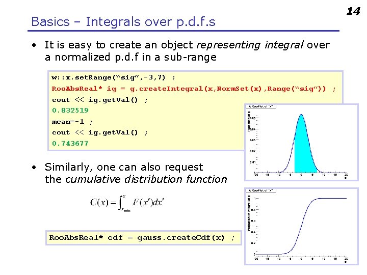
Basics – Integrals over p. d. f. s • It is easy to create an object representing integral over a normalized p. d. f in a sub-range w: : x. set. Range(“sig”, -3, 7) ; Roo. Abs. Real* ig = g. create. Integral(x, Norm. Set(x), Range(“sig”)) ; cout << ig. get. Val() ; 0. 832519 mean=-1 ; cout << ig. get. Val() ; 0. 743677 • Similarly, one can also request the cumulative distribution function Roo. Abs. Real* cdf = gauss. create. Cdf(x) ; 14

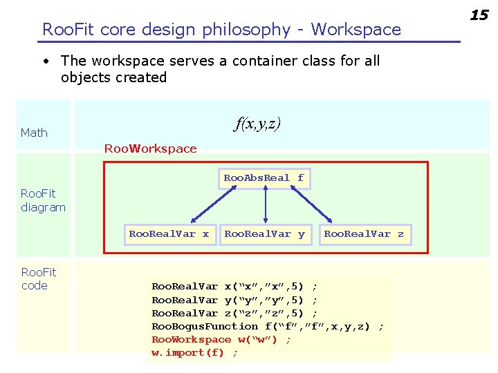
Roo. Fit core design philosophy - Workspace • The workspace serves a container class for all objects created f(x, y, z) Math Roo. Workspace Roo. Abs. Real f Roo. Fit diagram Roo. Real. Var x Roo. Fit code Roo. Real. Var y Roo. Real. Var z Roo. Real. Var x(“x”, ”x”, 5) ; Roo. Real. Var y(“y”, ”y”, 5) ; Roo. Real. Var z(“z”, ”z”, 5) ; Roo. Bogus. Function f(“f”, ”f”, x, y, z) ; Roo. Workspace w(“w”) ; w. import(f) ; 15

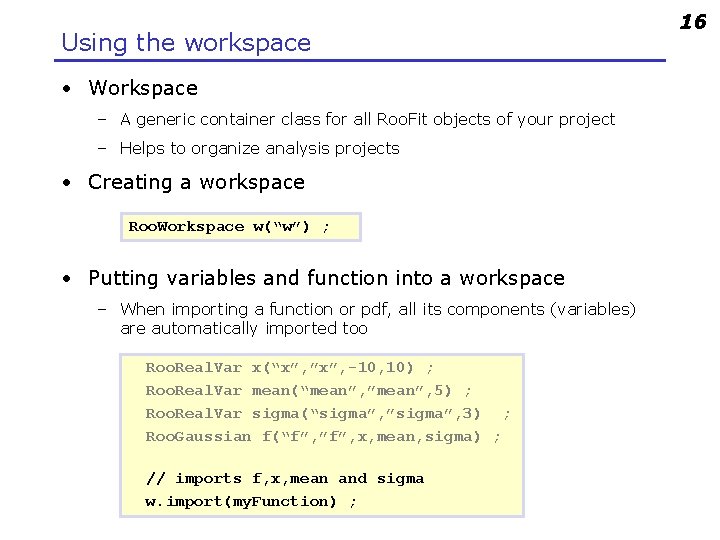
Using the workspace • Workspace – A generic container class for all Roo. Fit objects of your project – Helps to organize analysis projects • Creating a workspace Roo. Workspace w(“w”) ; • Putting variables and function into a workspace – When importing a function or pdf, all its components (variables) are automatically imported too Roo. Real. Var x(“x”, ”x”, -10, 10) ; Roo. Real. Var mean(“mean”, ”mean”, 5) ; Roo. Real. Var sigma(“sigma”, ”sigma”, 3) ; Roo. Gaussian f(“f”, ”f”, x, mean, sigma) ; // imports f, x, mean and sigma w. import(my. Function) ; 16

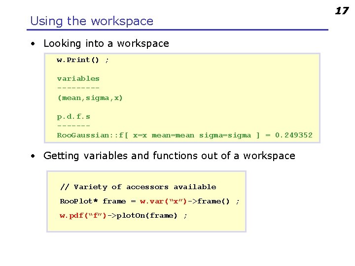
Using the workspace • Looking into a workspace w. Print() ; variables ----(mean, sigma, x) p. d. f. s ------Roo. Gaussian: : f[ x=x mean=mean sigma=sigma ] = 0. 249352 • Getting variables and functions out of a workspace // Variety of accessors available Roo. Plot* frame = w. var(“x”)->frame() ; w. pdf(“f”)->plot. On(frame) ; 17

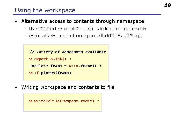
Using the workspace • Alternative access to contents through namespace – Uses CINT extension of C++, works in interpreted code only – (Alternatively construct workspace with k. TRUE as 2 nd arg) // Variety of accessors available w. export. To. Cint() ; Roo. Plot* frame = w: : x. frame() ; w: : f. plot. On(frame) ; • Writing workspace and contents to file w. write. To. File(“wspace. root”) ; 18

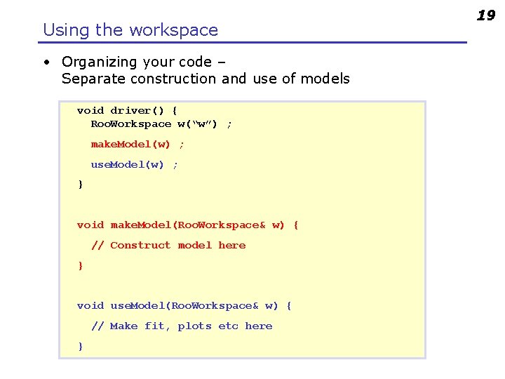
Using the workspace • Organizing your code – Separate construction and use of models void driver() { Roo. Workspace w(“w”) ; make. Model(w) ; use. Model(w) ; } void make. Model(Roo. Workspace& w) { // Construct model here } void use. Model(Roo. Workspace& w) { // Make fit, plots etc here } 19

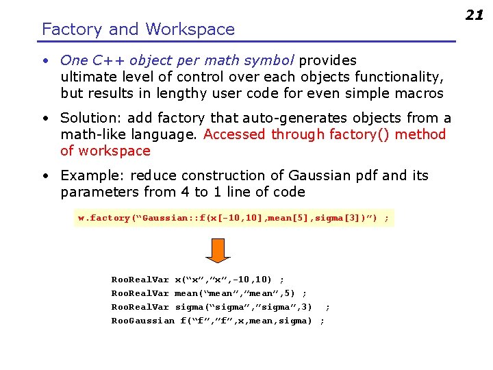
Factory and Workspace • One C++ object per math symbol provides ultimate level of control over each objects functionality, but results in lengthy user code for even simple macros • Solution: add factory that auto-generates objects from a math-like language. Accessed through factory() method of workspace • Example: reduce construction of Gaussian pdf and its parameters from 4 to 1 line of code w. factory(“Gaussian: : f(x[-10, 10], mean[5], sigma[3])”) ; Roo. Real. Var x(“x”, ”x”, -10, 10) ; Roo. Real. Var mean(“mean”, ”mean”, 5) ; Roo. Real. Var sigma(“sigma”, ”sigma”, 3) ; Roo. Gaussian f(“f”, ”f”, x, mean, sigma) ; 21

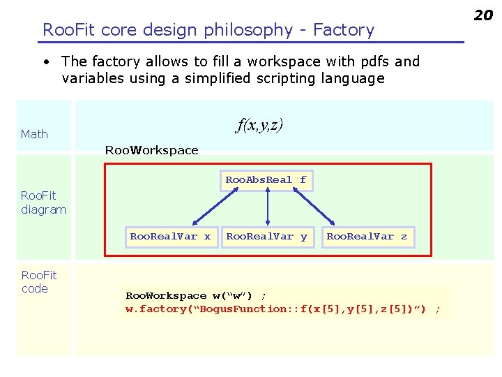
Roo. Fit core design philosophy - Factory • The factory allows to fill a workspace with pdfs and variables using a simplified scripting language f(x, y, z) Math Roo. Workspace Roo. Abs. Real f Roo. Fit diagram Roo. Real. Var x Roo. Fit code Roo. Real. Var y Roo. Real. Var z Roo. Workspace w(“w”) ; w. factory(“Bogus. Function: : f(x[5], y[5], z[5])”) ; 20

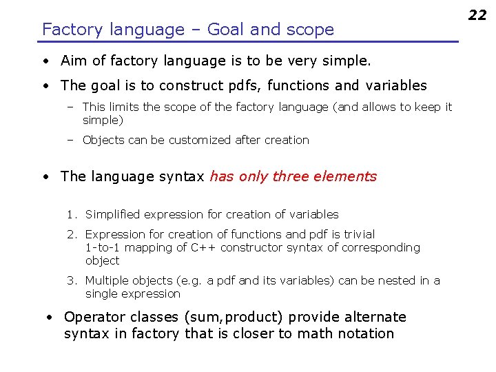
Factory language – Goal and scope • Aim of factory language is to be very simple. • The goal is to construct pdfs, functions and variables – This limits the scope of the factory language (and allows to keep it simple) – Objects can be customized after creation • The language syntax has only three elements 1. Simplified expression for creation of variables 2. Expression for creation of functions and pdf is trivial 1 -to-1 mapping of C++ constructor syntax of corresponding object 3. Multiple objects (e. g. a pdf and its variables) can be nested in a single expression • Operator classes (sum, product) provide alternate syntax in factory that is closer to math notation 22

Factory syntax 23 • Rule #1 – Create a variable x[-10, 10] // Create variable with given range x[5, -10, 10] // Create variable with initial value and range x[5] // Create initially constant variable • Rule #2 – Create a function or pdf object Class. Name: : Objectname(arg 1, [arg 2], . . . ) – Leading ‘Roo’ in class name can be omitted – Arguments are names of objects that already exist in the workspace – Named objects must be of correct type, if not factory issues error – Set and List arguments can be constructed with brackets {} Gaussian: : g(x, mean, sigma) Roo. Gaussian(“g”, ”g”, x, mean, sigma) Polynomial: : p(x, {a 0, a 1}) Roo. Polynomial(“p”, ”p”, x”, Roo. Arg. List(a 0, a 1));

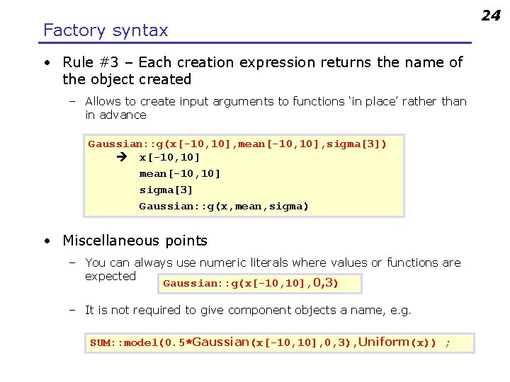
Factory syntax • Rule #3 – Each creation expression returns the name of the object created – Allows to create input arguments to functions ‘in place’ rather than in advance Gaussian: : g(x[-10, 10], mean[-10, 10], sigma[3]) x[-10, 10] mean[-10, 10] sigma[3] Gaussian: : g(x, mean, sigma) • Miscellaneous points – You can always use numeric literals where values or functions are expected Gaussian: : g(x[-10, 10], 0, 3) – It is not required to give component objects a name, e. g. SUM: : model(0. 5*Gaussian(x[-10, 10], 0, 3), Uniform(x)) ; 24

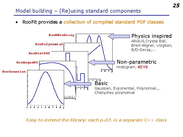
Model building – (Re)using standard components • Roo. Fit provides a collection of compiled standard PDF classes Physics inspired Roo. BMix. Decay ARGUS, Crystal Ball, Breit-Wigner, Voigtian, B/D-Decay, …. Roo. Polynomial Roo. Hist. Pdf Non-parametric Roo. Argus. BG Histogram, KEYS Roo. Gaussian Basic Gaussian, Exponential, Polynomial, … Chebychev polynomial Easy to extend the library: each p. d. f. is a separate C++ class 25

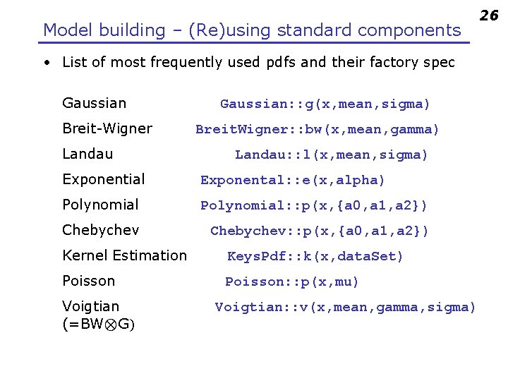
Model building – (Re)using standard components • List of most frequently used pdfs and their factory spec Gaussian Breit-Wigner Landau Gaussian: : g(x, mean, sigma) Breit. Wigner: : bw(x, mean, gamma) Landau: : l(x, mean, sigma) Exponential Exponental: : e(x, alpha) Polynomial: : p(x, {a 0, a 1, a 2}) Chebychev: : p(x, {a 0, a 1, a 2}) Kernel Estimation Keys. Pdf: : k(x, data. Set) Poisson: : p(x, mu) Voigtian (=BW⊗G) Voigtian: : v(x, mean, gamma, sigma) 26

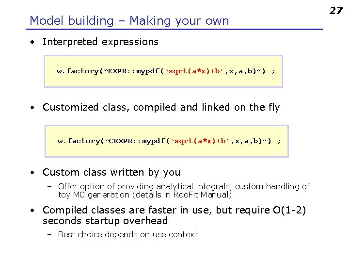
Model building – Making your own • Interpreted expressions w. factory(“EXPR: : mypdf(‘sqrt(a*x)+b’, x, a, b)”) ; • Customized class, compiled and linked on the fly w. factory(“CEXPR: : mypdf(‘sqrt(a*x)+b’, x, a, b)”) ; • Custom class written by you – Offer option of providing analytical integrals, custom handling of toy MC generation (details in Roo. Fit Manual) • Compiled classes are faster in use, but require O(1 -2) seconds startup overhead – Best choice depends on use context 27

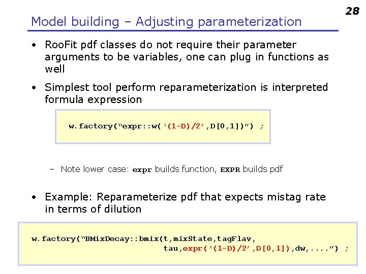
Model building – Adjusting parameterization 28 • Roo. Fit pdf classes do not require their parameter arguments to be variables, one can plug in functions as well • Simplest tool perform reparameterization is interpreted formula expression w. factory(“expr: : w(‘(1 -D)/2’, D[0, 1])”) ; – Note lower case: expr builds function, EXPR builds pdf • Example: Reparameterize pdf that expects mistag rate in terms of dilution w. factory(“BMix. Decay: : bmix(t, mix. State, tag. Flav, tau, expr(‘(1 -D)/2’, D[0, 1]), dw, . . ”) ;

3 Composite models

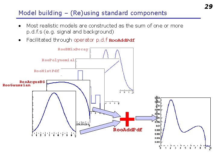
Model building – (Re)using standard components • Most realistic models are constructed as the sum of one or more p. d. f. s (e. g. signal and background) • Facilitated through operator p. d. f Roo. Add. Pdf Roo. BMix. Decay Roo. Polynomial Roo. Hist. Pdf Roo. Argus. BG Roo. Gaussian + Roo. Add. Pdf 29

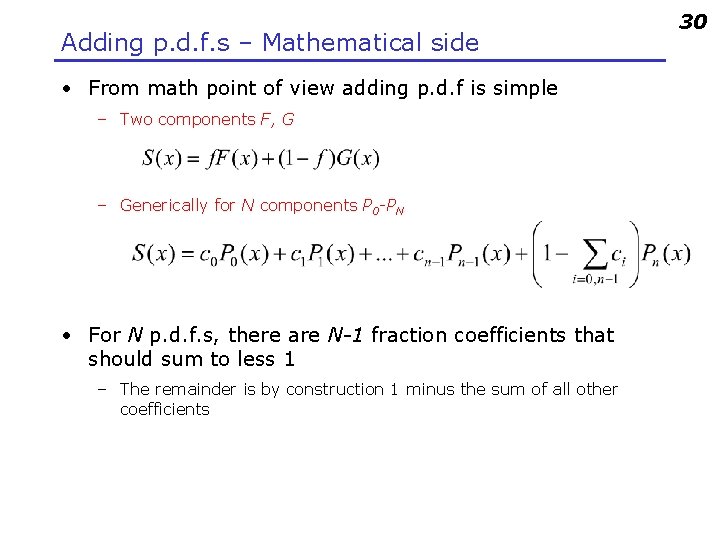
Adding p. d. f. s – Mathematical side • From math point of view adding p. d. f is simple – Two components F, G – Generically for N components P 0 -PN • For N p. d. f. s, there are N-1 fraction coefficients that should sum to less 1 – The remainder is by construction 1 minus the sum of all other coefficients 30

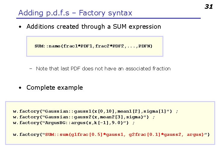
Adding p. d. f. s – Factory syntax 31 • Additions created through a SUM expression SUM: : name(frac 1*PDF 1, frac 2*PDF 2, . . . , PDFN) – Note that last PDF does not have an associated fraction • Complete example w. factory(“Gaussian: : gauss 1(x[0, 10], mean 1[2], sigma[1]”) ; w. factory(“Gaussian: : gauss 2(x, mean 2[3], sigma)”) ; w. factory(“Argus. BG: : argus(x, k[-1], 9. 0)”) ; w. factory(“SUM: : sum(g 1 frac[0. 5]*gauss 1, g 2 frac[0. 1]*gauss 2, argus)”)

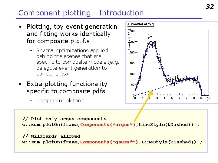
Component plotting - Introduction • Plotting, toy event generation and fitting works identically for composite p. d. f. s – Several optimizations applied behind the scenes that are specific to composite models (e. g. delegate event generation to components) • Extra plotting functionality specific to composite pdfs – Component plotting // Plot only argus components w: : sum. plot. On(frame, Components(“argus”), Line. Style(k. Dashed)) ; // Wildcards allowed w: : sum. plot. On(frame, Components(“gauss*”), Line. Style(k. Dashed)) ; 32

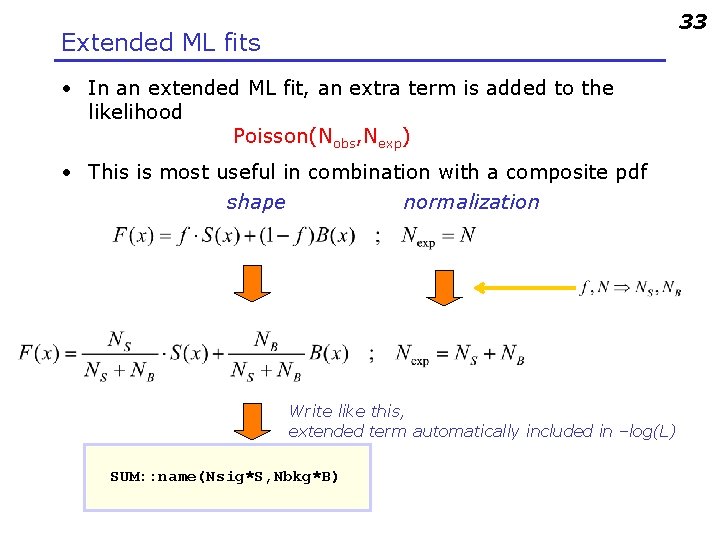
33 Extended ML fits • In an extended ML fit, an extra term is added to the likelihood Poisson(Nobs, Nexp) • This is most useful in combination with a composite pdf shape normalization Write like this, extended term automatically included in –log(L) SUM: : name(Nsig*S, Nbkg*B)

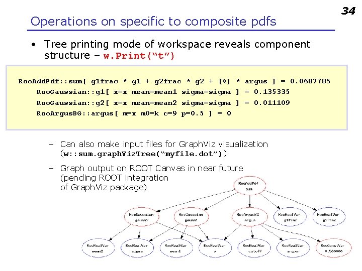
Operations on specific to composite pdfs • Tree printing mode of workspace reveals component structure – w. Print(“t”) Roo. Add. Pdf: : sum[ g 1 frac * g 1 + g 2 frac * g 2 + [%] * argus ] = 0. 0687785 Roo. Gaussian: : g 1[ x=x mean=mean 1 sigma=sigma ] = 0. 135335 Roo. Gaussian: : g 2[ x=x mean=mean 2 sigma=sigma ] = 0. 011109 Roo. Argus. BG: : argus[ m=x m 0=k c=9 p=0. 5 ] = 0 – Can also make input files for Graph. Viz visualization (w: : sum. graph. Viz. Tree(“myfile. dot”)) – Graph output on ROOT Canvas in near future (pending ROOT integration of Graph. Viz package) 34

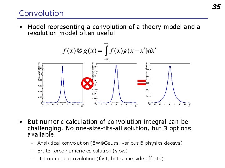
35 Convolution • Model representing a convolution of a theory model and a resolution model often useful = • But numeric calculation of convolution integral can be challenging. No one-size-fits-all solution, but 3 options available – Analytical convolution (BW Gauss, various B physics decays) – Brute-force numeric calculation (slow) – FFT numeric convolution (fast, but some side effects)

Convolution • Example w. factory(“Landau: : L(x[-10, 30], 5, 1)”) : w. factory(“Gaussian: : G(x, 0, 2)”) ; w: : x. set. Bins(“cache”, 10000) ; // FFT sampling density w. factory(“FCONV: : LGf(x, L, G)”) ; // FFT convolution w. factory(“NCONV: : LGb(x, L, G)”) ; // Numeric convolution • FFT usually best – Fast: unbinned ML fit to 10 K events take ~5 seconds – NB: Requires installation of FFTW package (free, but not default) – Beware of cyclical effects (some tools available to mitigate) 36

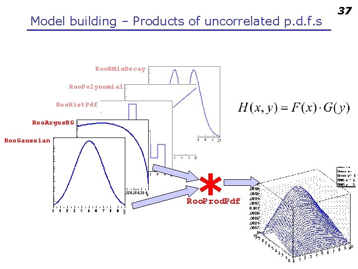
Model building – Products of uncorrelated p. d. f. s Roo. BMix. Decay Roo. Polynomial Roo. Hist. Pdf Roo. Argus. BG Roo. Gaussian * Roo. Prod. Pdf 37

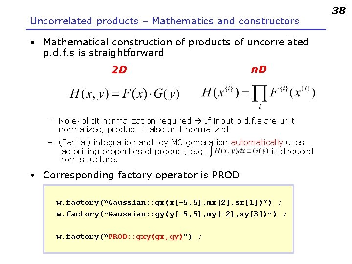
Uncorrelated products – Mathematics and constructors • Mathematical construction of products of uncorrelated p. d. f. s is straightforward 2 D n. D – No explicit normalization required If input p. d. f. s are unit normalized, product is also unit normalized – (Partial) integration and toy MC generation automatically uses factorizing properties of product, e. g. is deduced from structure. • Corresponding factory operator is PROD w. factory(“Gaussian: : gx(x[-5, 5], mx[2], sx[1])”) ; w. factory(“Gaussian: : gy(y[-5, 5], my[-2], sy[3])”) ; w. factory(“PROD: : gxy(gx, gy)”) ; 38

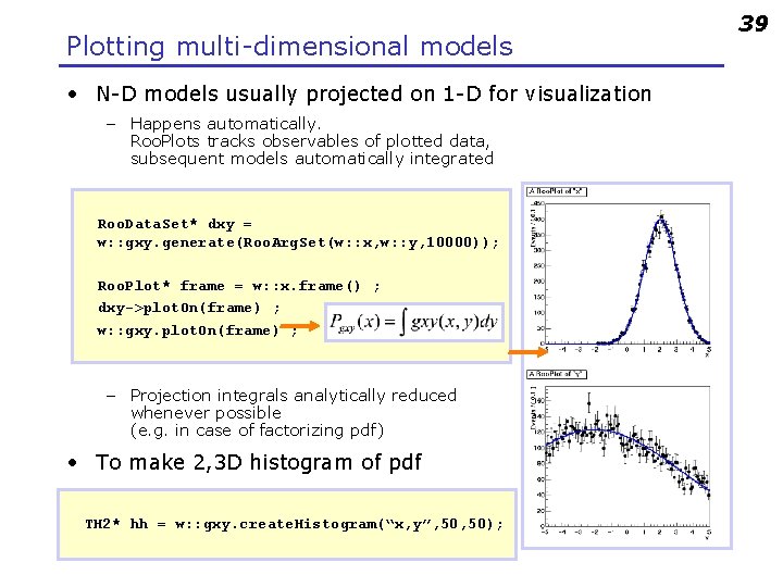
Plotting multi-dimensional models • N-D models usually projected on 1 -D for visualization – Happens automatically. Roo. Plots tracks observables of plotted data, subsequent models automatically integrated Roo. Data. Set* dxy = w: : gxy. generate(Roo. Arg. Set(w: : x, w: : y, 10000)); Roo. Plot* frame = w: : x. frame() ; dxy->plot. On(frame) ; w: : gxy. plot. On(frame) ; – Projection integrals analytically reduced whenever possible (e. g. in case of factorizing pdf) • To make 2, 3 D histogram of pdf TH 2* hh = w: : gxy. create. Histogram(“x, y”, 50); 39

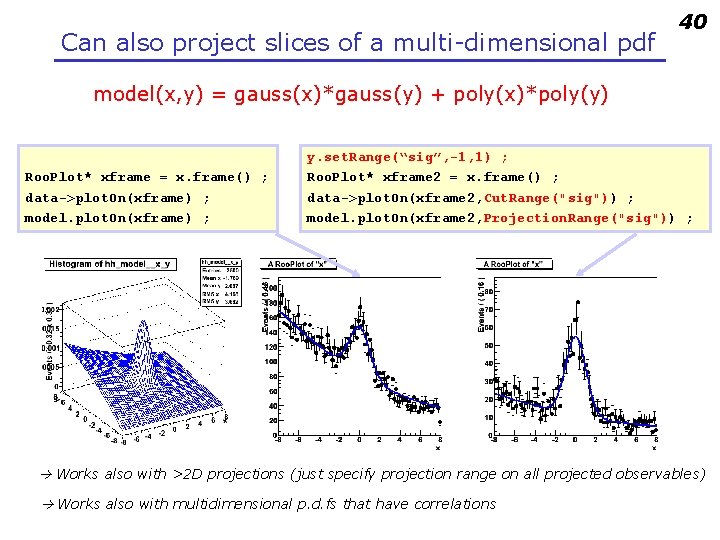
Can also project slices of a multi-dimensional pdf 40 model(x, y) = gauss(x)*gauss(y) + poly(x)*poly(y) Roo. Plot* xframe = x. frame() ; data->plot. On(xframe) ; model. plot. On(xframe) ; y. set. Range(“sig”, -1, 1) ; Roo. Plot* xframe 2 = x. frame() ; data->plot. On(xframe 2, Cut. Range("sig")) ; model. plot. On(xframe 2, Projection. Range("sig")) ; Works also with >2 D projections (just specify projection range on all projected observables) Works also with multidimensional p. d. fs that have correlations

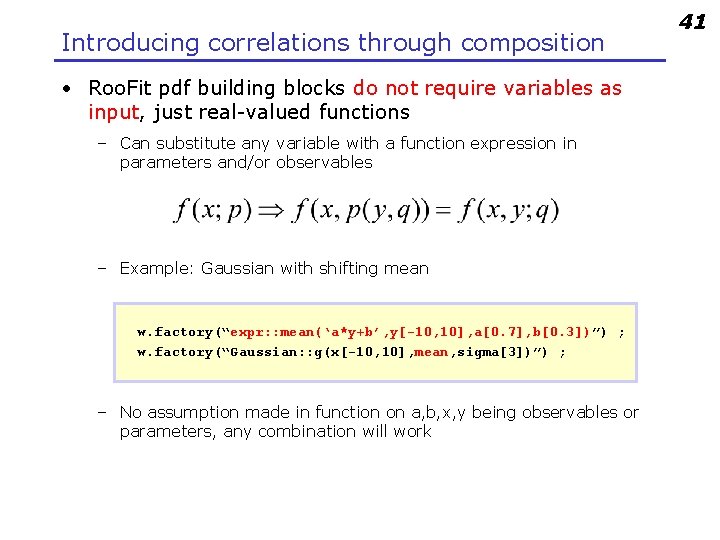
Introducing correlations through composition • Roo. Fit pdf building blocks do not require variables as input, just real-valued functions – Can substitute any variable with a function expression in parameters and/or observables – Example: Gaussian with shifting mean w. factory(“expr: : mean(‘a*y+b’, y[-10, 10], a[0. 7], b[0. 3])”) ; w. factory(“Gaussian: : g(x[-10, 10], mean, sigma[3])”) ; – No assumption made in function on a, b, x, y being observables or parameters, any combination will work 41

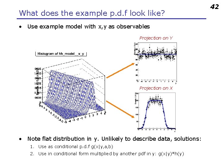
What does the example p. d. f look like? • Use example model with x, y as observables Projection on Y Projection on X • Note flat distribution in y. Unlikely to describe data, solutions: 1. Use as conditional p. d. f g(x|y, a, b) 2. Use in conditional form multiplied by another pdf in y: g(x|y)*h(y) 42

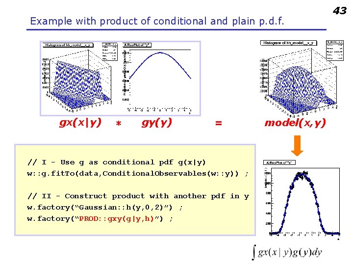
Example with product of conditional and plain p. d. f. gx(x|y) * gy(y) = // I - Use g as conditional pdf g(x|y) w: : g. fit. To(data, Conditional. Observables(w: : y)) ; // II - Construct product with another pdf in y w. factory(“Gaussian: : h(y, 0, 2)”) ; w. factory(“PROD: : gxy(g|y, h)”) ; model(x, y) 43

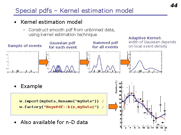
Special pdfs – Kernel estimation model 44 • Kernel estimation model – Construct smooth pdf from unbinned data, using kernel estimation technique Sample of events Gaussian pdf for each event Summed pdf for all events • Example w. import(my. Data, Rename(“my. Data”)) ; w. factory(“Keys. Pdf: : k(x, my. Data)”) ; • Also available for n-D data Adaptive Kernel: width of Gaussian depends on local event density

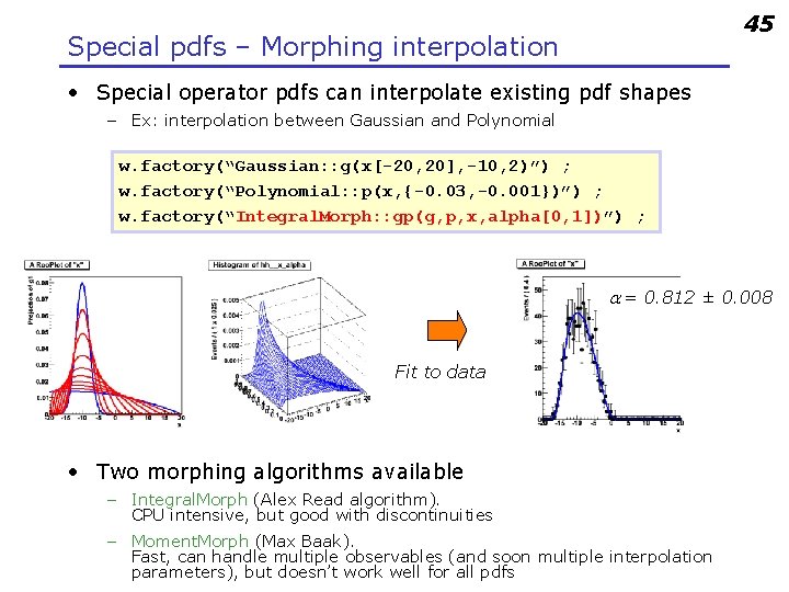
45 Special pdfs – Morphing interpolation • Special operator pdfs can interpolate existing pdf shapes – Ex: interpolation between Gaussian and Polynomial w. factory(“Gaussian: : g(x[-20, 20], -10, 2)”) ; w. factory(“Polynomial: : p(x, {-0. 03, -0. 001})”) ; w. factory(“Integral. Morph: : gp(g, p, x, alpha[0, 1])”) ; a = 0. 812 ± 0. 008 Fit to data • Two morphing algorithms available – Integral. Morph (Alex Read algorithm). CPU intensive, but good with discontinuities – Moment. Morph (Max Baak). Fast, can handle multiple observables (and soon multiple interpolation parameters), but doesn’t work well for all pdfs

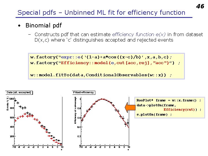
Special pdfs – Unbinned ML fit for efficiency function 46 • Binomial pdf – Constructs pdf that can estimate efficiency function e(x) in from dataset D(x, c) where ‘c’ distinguishes accepted and rejected events w. factory(“expr: : e(‘(1 -a)+a*cos((x-c)/b)’, x, a, b, c); w. factory(“Efficiency: : model(e, cut[acc, rej], "acc")”) ; w: : model. fit. To(data, Conditional. Observables(w: : x)) ; Roo. Plot* frame = w: : x. frame() ; data->plot. On(frame, Efficiency(cut)) ; e. plot. On(frame) ;

4 Likelihood & Profile Likelihood

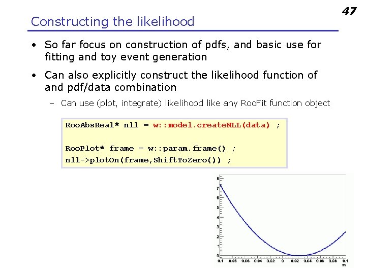
Constructing the likelihood • So far focus on construction of pdfs, and basic use for fitting and toy event generation • Can also explicitly construct the likelihood function of and pdf/data combination – Can use (plot, integrate) likelihood like any Roo. Fit function object Roo. Abs. Real* nll = w: : model. create. NLL(data) ; Roo. Plot* frame = w: : param. frame() ; nll->plot. On(frame, Shift. To. Zero()) ; 47

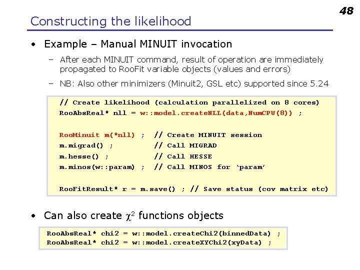
Constructing the likelihood • Example – Manual MINUIT invocation – After each MINUIT command, result of operation are immediately propagated to Roo. Fit variable objects (values and errors) – NB: Also other minimizers (Minuit 2, GSL etc) supported since 5. 24 // Create likelihood (calculation parallelized on 8 cores) Roo. Abs. Real* nll = w: : model. create. NLL(data, Num. CPU(8)) ; Roo. Minuit m(*nll) ; m. migrad() ; m. hesse() ; m. minos(w: : param) ; // // Create MINUIT session Call MIGRAD Call HESSE Call MINOS for ‘param’ Roo. Fit. Result* r = m. save() ; // Save status (cov matrix etc) • Can also create c 2 functions objects Roo. Abs. Real* chi 2 = w: : model. create. Chi 2(binned. Data) ; Roo. Abs. Real* chi 2 = w: : model. create. XYChi 2(xy. Data) ; 48

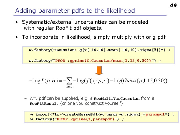
Adding parameter pdfs to the likelihood 49 • Systematic/external uncertainties can be modeled with regular Roo. Fit pdf objects. • To incorporate in likelihood, simply multiply with orig pdf w. factory(“Gaussian: : g(x[-10, 10], mean[-10, 10], sigma[3])”) ; w. factory(“PROD: : gprime(f, Gaussian(mean, 1. 15, 0. 30))”) ; – Any pdf can be supplied, e. g. a Roo. Multi. Var. Gaussian from a Roo. Fit. Result (or one you construct yourself) w. import(*fr->create. Hesse. Pdf(w: : mean, w: : sigma), ”parampdf”) ; w. factory(“PROD: : gprime(f, parampdf)”) ;

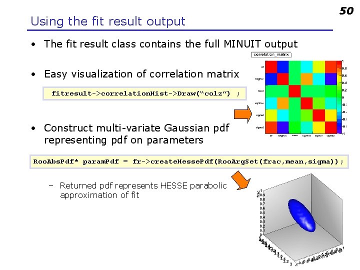
Using the fit result output 50 • The fit result class contains the full MINUIT output • Easy visualization of correlation matrix fitresult->correlation. Hist->Draw(“colz”) ; • Construct multi-variate Gaussian pdf representing pdf on parameters Roo. Abs. Pdf* param. Pdf = fr->create. Hesse. Pdf(Roo. Arg. Set(frac, mean, sigma)); – Returned pdf represents HESSE parabolic approximation of fit

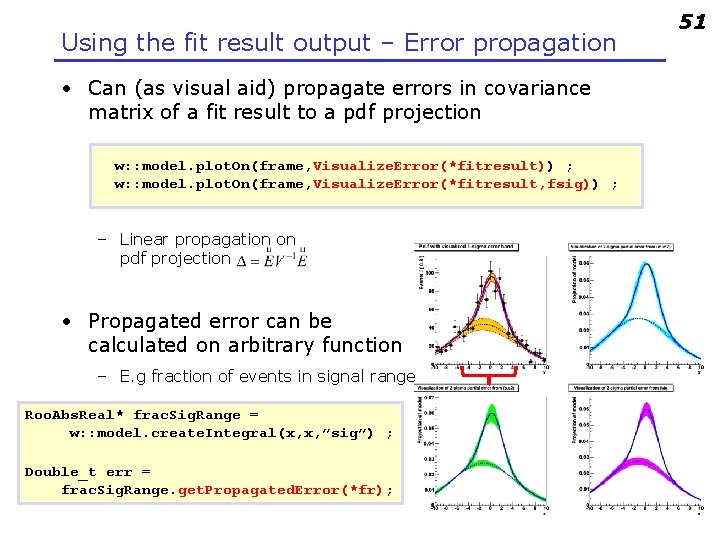
Using the fit result output – Error propagation • Can (as visual aid) propagate errors in covariance matrix of a fit result to a pdf projection w: : model. plot. On(frame, Visualize. Error(*fitresult)) ; w: : model. plot. On(frame, Visualize. Error(*fitresult, fsig)) ; – Linear propagation on pdf projection • Propagated error can be calculated on arbitrary function – E. g fraction of events in signal range Roo. Abs. Real* frac. Sig. Range = w: : model. create. Integral(x, x, ”sig”) ; Double_t err = frac. Sig. Range. get. Propagated. Error(*fr); 51

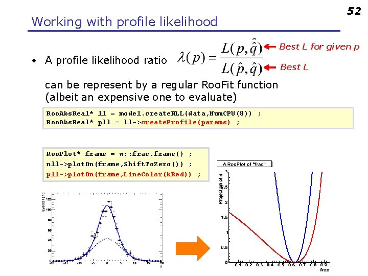
52 Working with profile likelihood Best L for given p • A profile likelihood ratio can be represent by a regular Roo. Fit function (albeit an expensive one to evaluate) Roo. Abs. Real* ll = model. create. NLL(data, Num. CPU(8)) ; Roo. Abs. Real* pll = ll->create. Profile(params) ; Roo. Plot* frame = w: : frac. frame() ; nll->plot. On(frame, Shift. To. Zero()) ; pll->plot. On(frame, Line. Color(k. Red)) ; Best L

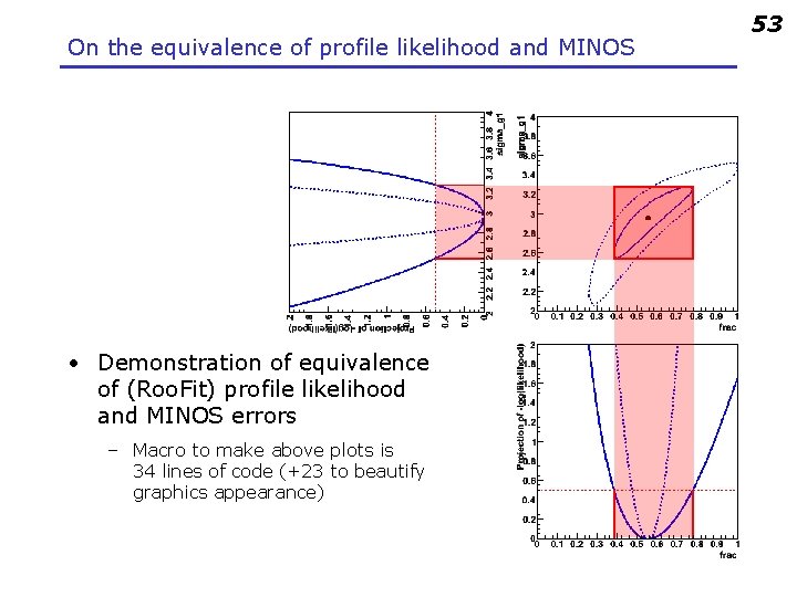
On the equivalence of profile likelihood and MINOS • Demonstration of equivalence of (Roo. Fit) profile likelihood and MINOS errors – Macro to make above plots is 34 lines of code (+23 to beautify graphics appearance) 53

5 Simultaneous fits and combinations

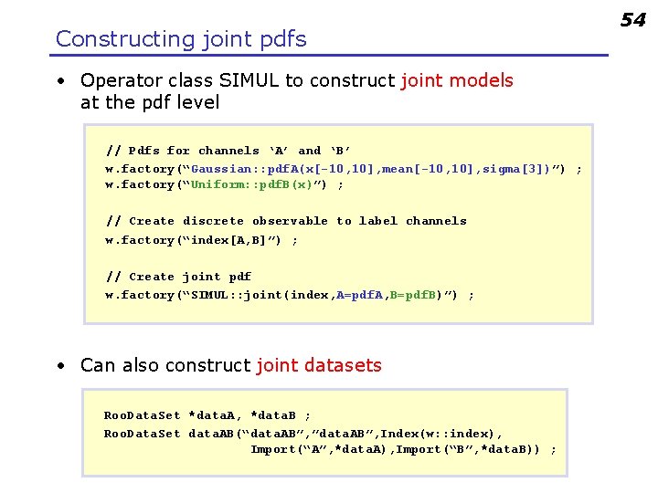
Constructing joint pdfs • Operator class SIMUL to construct joint models at the pdf level // Pdfs for channels ‘A’ and ‘B’ w. factory(“Gaussian: : pdf. A(x[-10, 10], mean[-10, 10], sigma[3])”) ; w. factory(“Uniform: : pdf. B(x)”) ; // Create discrete observable to label channels w. factory(“index[A, B]”) ; // Create joint pdf w. factory(“SIMUL: : joint(index, A=pdf. A, B=pdf. B)”) ; • Can also construct joint datasets Roo. Data. Set *data. A, *data. B ; Roo. Data. Set data. AB(“data. AB”, ”data. AB”, Index(w: : index), Import(“A”, *data. A), Import(“B”, *data. B)) ; 54

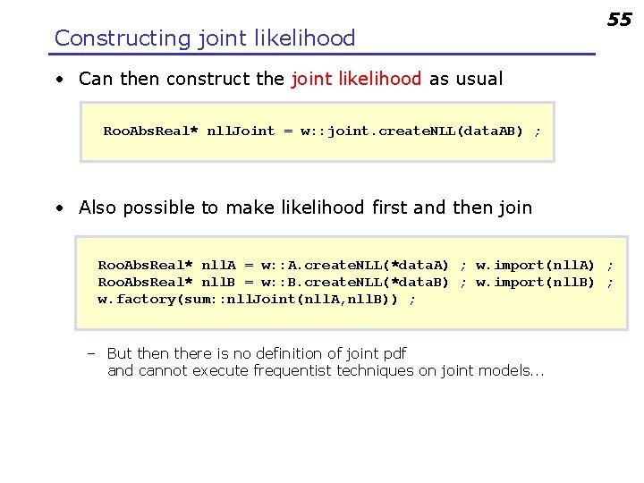
Constructing joint likelihood 55 • Can then construct the joint likelihood as usual Roo. Abs. Real* nll. Joint = w: : joint. create. NLL(data. AB) ; • Also possible to make likelihood first and then join Roo. Abs. Real* nll. A = w: : A. create. NLL(*data. A) ; w. import(nll. A) ; Roo. Abs. Real* nll. B = w: : B. create. NLL(*data. B) ; w. import(nll. B) ; w. factory(sum: : nll. Joint(nll. A, nll. B)) ; – But then there is no definition of joint pdf and cannot execute frequentist techniques on joint models. . .

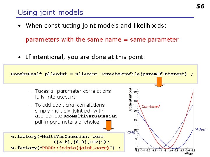
Using joint models • When constructing joint models and likelihoods: parameters with the same name = same parameter • If intentional, you are done at this point. Roo. Abs. Real* pll. Joint = nll. Joint->create. Profile(param. Of. Interest) ; – Takes all parameter correlations fully into account – To additional correlations, simply multiply joint pdf with appropriate Roo. Multi. Var. Gaussian pdf in parameters of choice w. factory(“Multi. Var. Gaussian: : corr ({a, b}, {0, 0}, COV)”); w. factory(“PROD: : jointc(joint, corr)”) ; 56

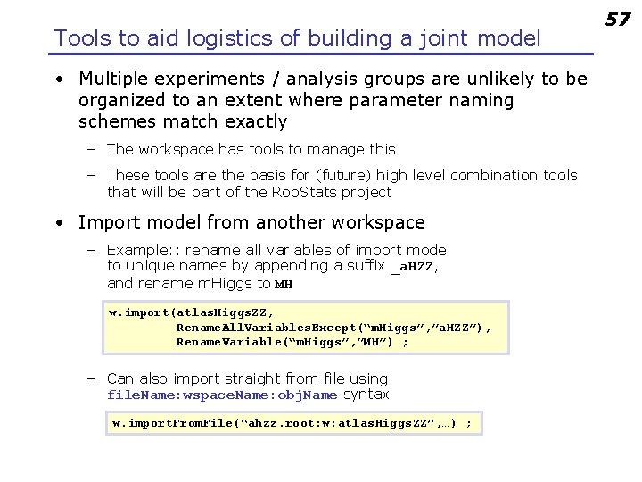
Tools to aid logistics of building a joint model • Multiple experiments / analysis groups are unlikely to be organized to an extent where parameter naming schemes match exactly – The workspace has tools to manage this – These tools are the basis for (future) high level combination tools that will be part of the Roo. Stats project • Import model from another workspace – Example: : rename all variables of import model to unique names by appending a suffix _a. HZZ, and rename m. Higgs to MH w. import(atlas. Higgs. ZZ, Rename. All. Variables. Except(“m. Higgs”, ”a. HZZ”), Rename. Variable(“m. Higgs”, ”MH”) ; – Can also import straight from file using file. Name: wspace. Name: obj. Name syntax w. import. From. File(“ahzz. root: w: atlas. Higgs. ZZ”, …) ; 57

Summary • Brief overview of Roo. Fit functionality, tailored to serve as introductory to Roo. Stats – Many features were not mentioned here – No discussion of how this work internally (optimization, analytical deduction abilities) – About 90% of the details were omitted • Documentation – Starting point: http: //root. cern. ch/drupal/content /roofit – Users manual (134 pages ~ 1 year old) – Quick Start Guide (20 pages, recent) – Link to 84 tutorial macros (also in $ROOTSYS/tutorials/roofit) • Support – Post your question on ‘Stat & Math Forum’ of ROOT (root. cern. ch Forum Stat & Math tools) – I aim for <24 h response (but I don’t manage every day!) 58

6 Hands-on exercises

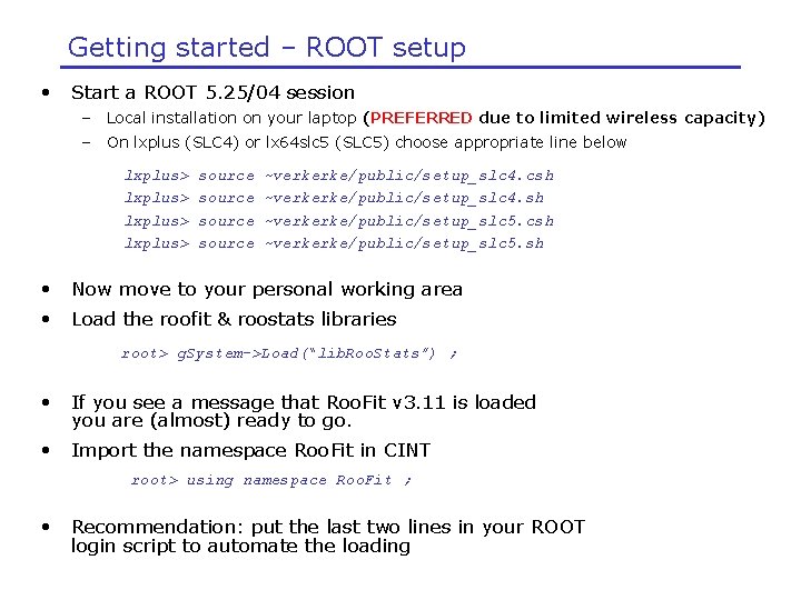
Getting started – ROOT setup • Start a ROOT 5. 25/04 session – Local installation on your laptop (PREFERRED due to limited wireless capacity) – On lxplus (SLC 4) or lx 64 slc 5 (SLC 5) choose appropriate line below lxplus> source ~verkerke/public/setup_slc 4. csh ~verkerke/public/setup_slc 4. sh ~verkerke/public/setup_slc 5. csh ~verkerke/public/setup_slc 5. sh • Now move to your personal working area • Load the roofit & roostats libraries root> g. System->Load(“lib. Roo. Stats”) ; • If you see a message that Roo. Fit v 3. 11 is loaded you are (almost) ready to go. • Import the namespace Roo. Fit in CINT root> using namespace Roo. Fit ; • Recommendation: put the last two lines in your ROOT login script to automate the loading

Getting started – Online reference material • Roo. Fit class documentation (from code) – http: //root. cern. ch/root/html/ROOFIT_ROOFITCORE_Index. html – http: //root. cern. ch/root/html/ROOFIT_Index. html • Roo. Fit home page at ROOT web site – http: //root. cern. ch/drupal/content/roofit – Has links to manual and tutorial macros

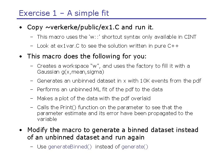
Exercise 1 – A simple fit • Copy ~verkerke/public/ex 1. C and run it. – This macro uses the ‘w: : ’ shortcut syntax only available in CINT – Look at ex 1 var. C to see the solution written in pure C++ • This macro does the following for you: – Creates a workspace “w”, and uses the factory to fill it with a Gaussian g(x, mean, sigma) – Generates an unbinned dataset in x with 10 K events from the pdf – Performs an unbinned ML fit of the pdf to the data – Makes a plot of the data with the pdf overlaid – Calls the Print() function on the parameter to see that the parameter estimate and its error have been propagated to the variable • Modify the macro to generate a binned dataset instead of an unbinned dataset and run again – Use generate. Binned() instead of generate()

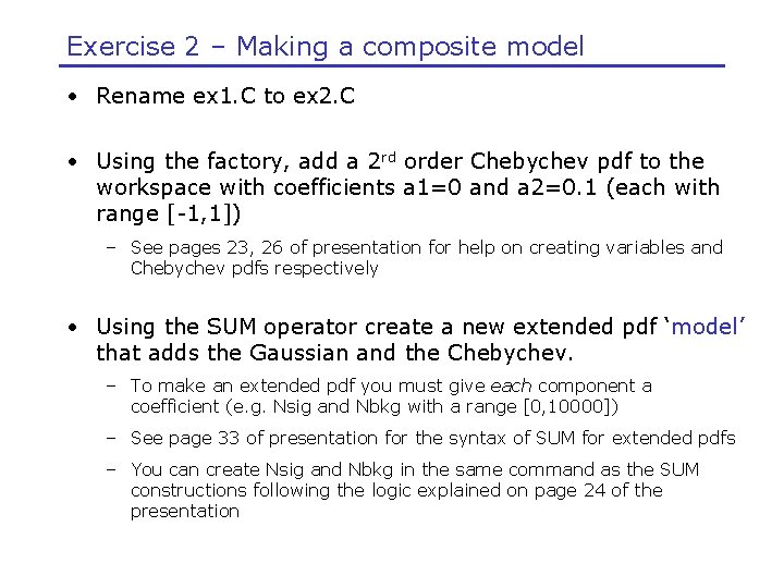
Exercise 2 – Making a composite model • Rename ex 1. C to ex 2. C • Using the factory, add a 2 rd order Chebychev pdf to the workspace with coefficients a 1=0 and a 2=0. 1 (each with range [-1, 1]) – See pages 23, 26 of presentation for help on creating variables and Chebychev pdfs respectively • Using the SUM operator create a new extended pdf ‘model’ that adds the Gaussian and the Chebychev. – To make an extended pdf you must give each component a coefficient (e. g. Nsig and Nbkg with a range [0, 10000]) – See page 33 of presentation for the syntax of SUM for extended pdfs – You can create Nsig and Nbkg in the same command as the SUM constructions following the logic explained on page 24 of the presentation

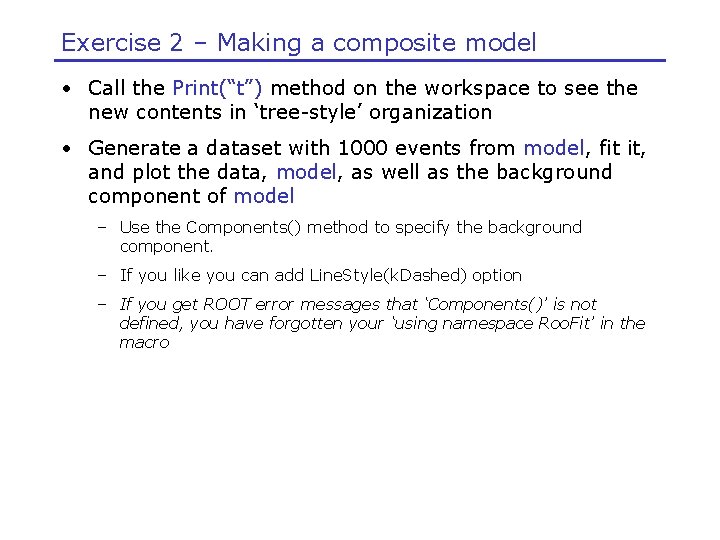
Exercise 2 – Making a composite model • Call the Print(“t”) method on the workspace to see the new contents in ‘tree-style’ organization • Generate a dataset with 1000 events from model, fit it, and plot the data, model, as well as the background component of model – Use the Components() method to specify the background component. – If you like you can add Line. Style(k. Dashed) option – If you get ROOT error messages that ‘Components()’ is not defined, you have forgotten your ‘using namespace Roo. Fit’ in the macro

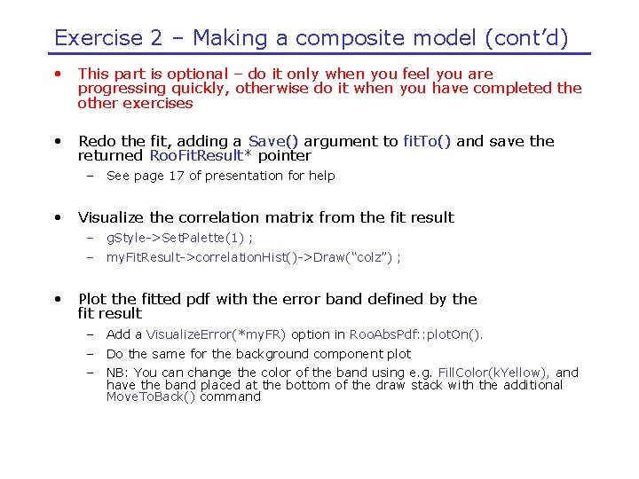
Exercise 2 – Making a composite model (cont’d) • This part is optional – do it only when you feel you are progressing quickly, otherwise do it when you have completed the other exercises • Redo the fit, adding a Save() argument to fit. To() and save the returned Roo. Fit. Result* pointer – See page 17 of presentation for help • Visualize the correlation matrix from the fit result – g. Style->Set. Palette(1) ; – my. Fit. Result->correlation. Hist()->Draw(“colz”) ; • Plot the fitted pdf with the error band defined by the fit result – Add a Visualize. Error(*my. FR) option in Roo. Abs. Pdf: : plot. On(). – Do the same for the background component plot – NB: You can change the color of the band using e. g. Fill. Color(k. Yellow), and have the band placed at the bottom of the draw stack with the additional Move. To. Back() command

Demo 1 – FFT convolution of arbitrary pdfs • Copy ~verkerke/public/fftdemo. C and run it • This macro demonstrates how the FCONV fourier convolution operator is used to convolute a Landau pdf with a Gaussian resolution model • A binned likelihood fit of the numerically convoluted pdf with three floating parameters takes ~1 second

Exercise 3 – Persisting your model • Copy ex 2. C to ex 3 a. C • At the end of the macro, import the toy data you generated into the workspace as follows – w. import(data, Rename(“data”)) ; • Write your workspace to file – using the method w. write. To. File(“model. root”). • Now quit your ROOT session • Copy ~verkerke/public/ex 3 b. C. – This macro will read in your model. root file and plot the pdf and dataset contained in it • Look at the macro and run it

Demo 2 – simultaneous fitting • Copy ~verkerke/public/simfitdemo. C and run it • This macro demonstrates techniques to make simultaneous fits to a ‘signal’ and ‘control’ samples in multiple ways 1. Plain fit of model sig. Pdf+bkg. Pdf to ‘signal sample’ 2. Plain fit of model sig. Pdf+bkg. Pdf. Ctrl to ‘control sample’ 3. A simultaneous fit of 1) and 2). – The determination of the parameters that occur in both model 1) and 2) are now determined from the joint likelihood fit – The uncertainty of the signal pdf shape is now noticeably smaller then when fitting 1) by itself 4. Express parabolic likelihood approximation of control sample fit (2) as pdf on sig. Pdf parameters , multiply likelihood of signal sample fit (1) with this pdf – Result is equivalent to 3) (in the limit that the actual likelihood of 2) is parabolic), but the ‘joint’ likelihood calculation is much faster than in 3) as the control sample likelihood is now parameterized

Exercise 4 – Working with the likelihood • Copy ex 3 b. C to ex 4. C • Remove the plotting code and add a line to create a function object that represents the –log(likelihood) – Use method Roo. Abs. Pdf: : create. NLL(Roo. Abs. Data&), the returned object is of type Roo. Abs. Real* – See page 47 in the presentation for help • Minimize the likelihood function ‘by hand’ by passing it to a Roo. Minuit object and calling its methods migrad() and hesse() – See page 48 in the presentation for help (also for below) – Now call the minos() function only for parameter Nsig. – Call w: : Nsig. Print() afterwards to see that the asymmetric error has been propagated – Fix the width of the Gaussian (use w: : sigma. set. Constant(k. TRUE)), run MINOS again and observe the effect.

Exercise 4 – Working with the likelihood • Make a plot of –log(L) vs Nsig – First create a plot frame in the parameter using Roo. Plot* frame = w: : Nsig. frame() ; – Now plot the likelihood function on the frame, using plot. On() as usual – If you like you can add a Shift. To. Zero() argument to the plot. On() call and see what that does – You can adjust the virtual range of the plot frame with Set. Minimum() and Set. Maximum().

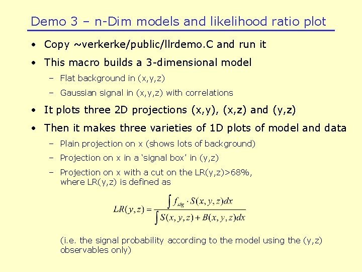
Demo 3 – n-Dim models and likelihood ratio plot • Copy ~verkerke/public/llrdemo. C and run it • This macro builds a 3 -dimensional model – Flat background in (x, y, z) – Gaussian signal in (x, y, z) with correlations • It plots three 2 D projections (x, y), (x, z) and (y, z) • Then it makes three varieties of 1 D plots of model and data – Plain projection on x (shows lots of background) – Projection on x in a ‘signal box’ in (y, z) – Projection on x with a cut on the LR(y, z)>68%, where LR(y, z) is defined as (i. e. the signal probability according to the model using the (y, z) observables only)

Exercise 5 – Profile likelihood • Copy ~verkerke/public/ex 4. C (standard solution to ex 4) to ex 5. C • Adjust the horizontal plot range of the likelihood plot so that it just covers the interval ΔLL=+25 units – Make a new plot frame that zooms in on that range and plot the likelihood again (you can specify myparam. frame(pmin, pmax) when you construct the plot frame to control the plot range) • Create the profile likelihood function in Nsig – Call method create. Profile(w: : Nsig) on the likelihood function object and save the returned pointer to the profile likelihood function (again of type Roo. Abs. Real*) – Plot the profile likelihood ratio on the Nsig frame too (make it red by adding a Line. Color(k. Red) to the plot. On() command) • Find the profile likelihood ratio interval of Nsig : find the points at which the PLR rises by +0. 5 units – Compare the interval to that of the MINOS error of exercise Ex 4.

Exercise 6 – Parallelizing the likelihood calculation • Check the number of CPU cores available on the current host (‘cat /proc/cpuinfo’) • Modify the create. NLL() call of ex 5 to take an extra Num. CPU(N) argument – The likelihood calculation will now be parallelized over N cores • Rerun ex 5 and observe the difference in wall-time execution speed. – The speedup is best demonstrated on an empty worker node (your best is lx 64 slc 5)