Recursive Sorting 15 211 Fundamental Data Structures and

Recursive Sorting 15 -211 Fundamental Data Structures and Algorithms Peter Lee October 23, 2001

Announcements § HW 4 due tonight! § Midterm exam on Thursday. ØIn class, one hour exam. ØOpen book, open notes. ØNo computers.

Recap

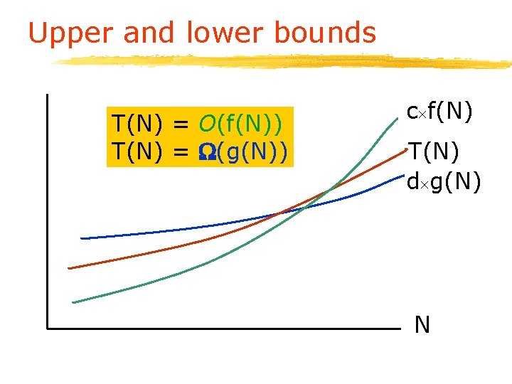
Upper and lower bounds T(N) = O(f(N)) T(N) = (g(N)) c f(N) T(N) d g(N) N

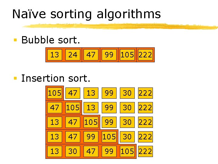
Naïve sorting algorithms § Bubble sort. 24 13 13 47 24 47 13 99 105 222 § Insertion sort. 105 47 13 99 30 222 47 105 13 99 30 222 13 47 105 99 30 222 13 47 99 105 30 222 13 30 47 99 105 222

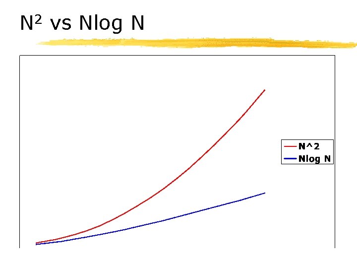
N 2 vs Nlog N

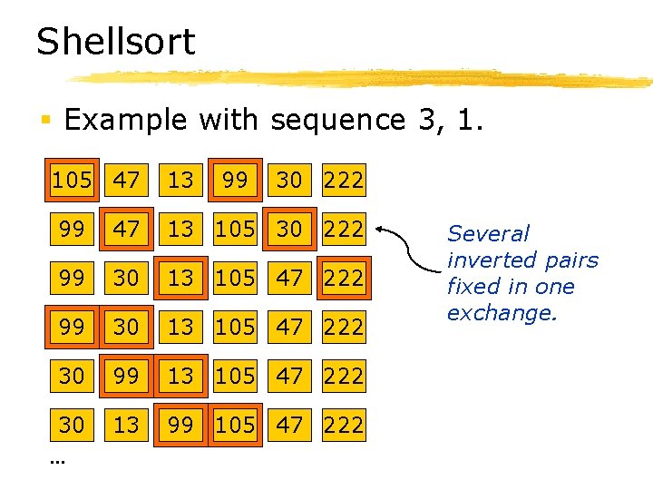
Shellsort § Example with sequence 3, 1. 105 47 13 99 30 222 99 47 13 105 30 222 99 30 13 105 47 222 30 99 13 105 47 222 30. . . 13 99 105 47 222 Several inverted pairs fixed in one exchange.

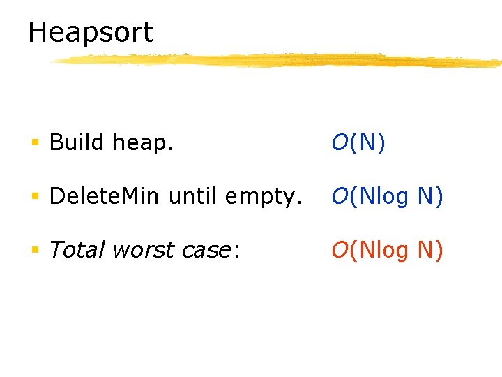
Heapsort § Build heap. O(N) § Delete. Min until empty. O(Nlog N) § Total worst case: O(Nlog N)

Recursive Sorting and Recurrence Relations

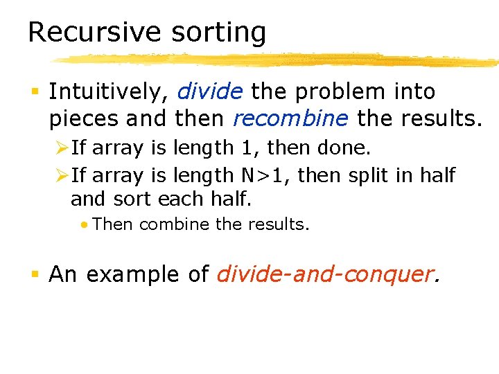
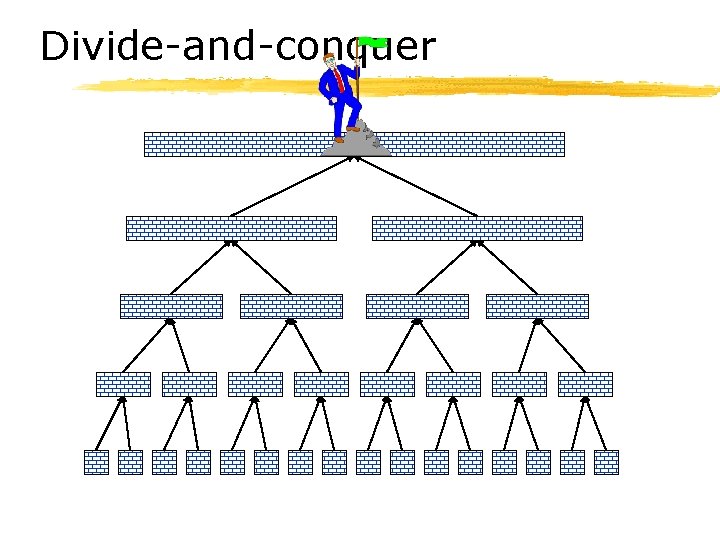
Recursive sorting § Intuitively, divide the problem into pieces and then recombine the results. ØIf array is length 1, then done. ØIf array is length N>1, then split in half and sort each half. • Then combine the results. § An example of divide-and-conquer.

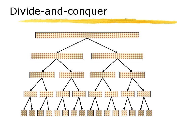
Divide-and-conquer

Divide-and-conquer

Why divide-and-conquer works § Suppose the amount of work required to divide and recombine is linear, that is, O(N). § Suppose also that the amount of work to complete each step is greater than linear. § Then each dividing step reduces the amount of work by greater than a linear amount, while requiring only linear work to do so.

Divide-and-conquer is big § We will see several examples of divide-and-conquer in this course.

Recursive sorting § If array is length 1, then done. § If array is length N>1, then split in half and sort each half. ØThen combine the results.

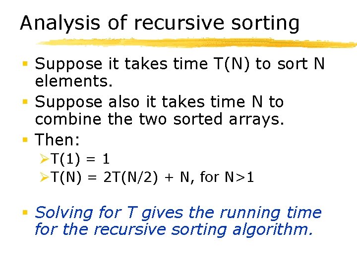
Analysis of recursive sorting § Suppose it takes time T(N) to sort N elements. § Suppose also it takes time N to combine the two sorted arrays. § Then: ØT(1) = 1 ØT(N) = 2 T(N/2) + N, for N>1 § Solving for T gives the running time for the recursive sorting algorithm.

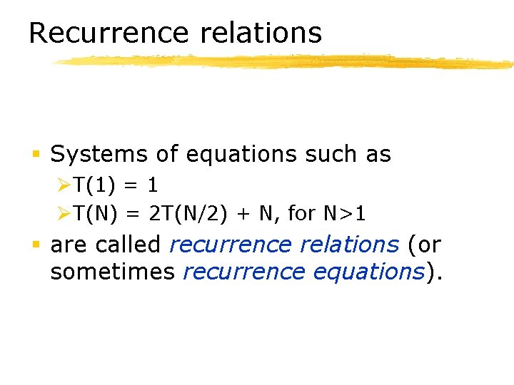
Recurrence relations § Systems of equations such as ØT(1) = 1 ØT(N) = 2 T(N/2) + N, for N>1 § are called recurrence relations (or sometimes recurrence equations).

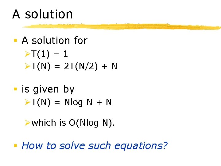
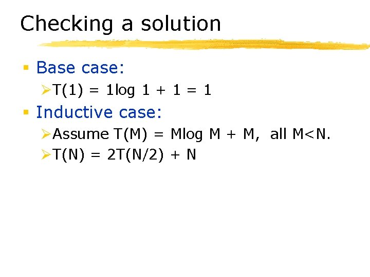
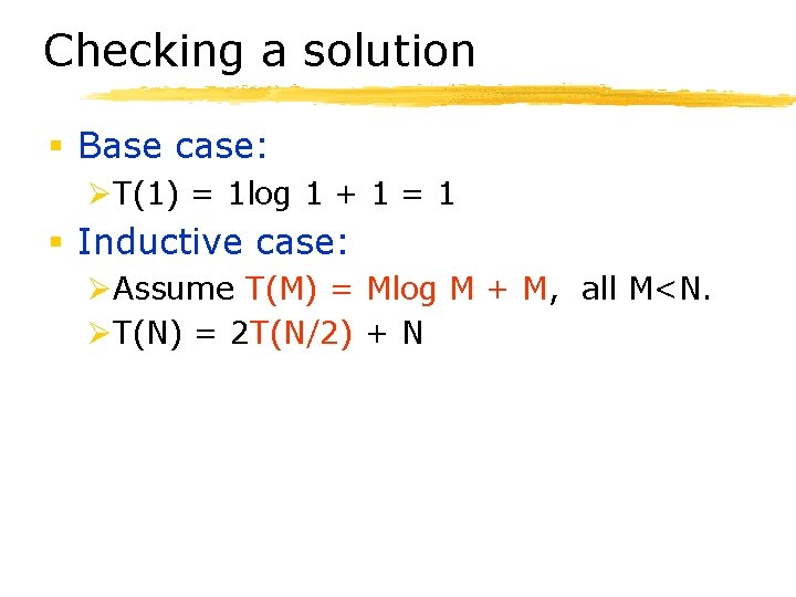
A solution § A solution for ØT(1) = 1 ØT(N) = 2 T(N/2) + N § is given by ØT(N) = Nlog N + N Øwhich is O(Nlog N). § How to solve such equations?

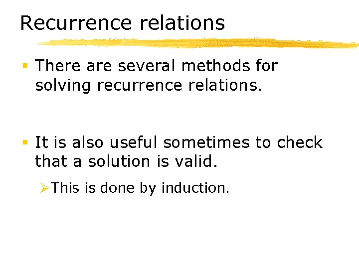
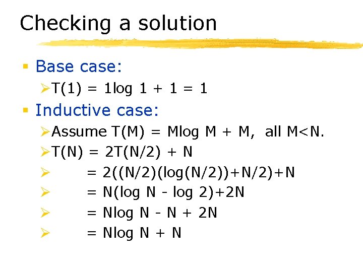
Recurrence relations § There are several methods for solving recurrence relations. § It is also useful sometimes to check that a solution is valid. ØThis is done by induction.

Checking a solution § Base case: ØT(1) = 1 log 1 + 1 = 1 § Inductive case: ØAssume T(M) = Mlog M + M, all M<N. ØT(N) = 2 T(N/2) + N

Checking a solution § Base case: ØT(1) = 1 log 1 + 1 = 1 § Inductive case: ØAssume T(M) = Mlog M + M, all M<N. ØT(N) = 2 T(N/2) + N

Checking a solution § Base case: ØT(1) = 1 log 1 + 1 = 1 § Inductive case: ØAssume T(M) = Mlog M + M, all M<N. ØT(N) = 2 T(N/2) + N Ø = 2((N/2)(log(N/2))+N/2)+N Ø = N(log N - log 2)+2 N Ø = Nlog N - N + 2 N Ø = Nlog N + N

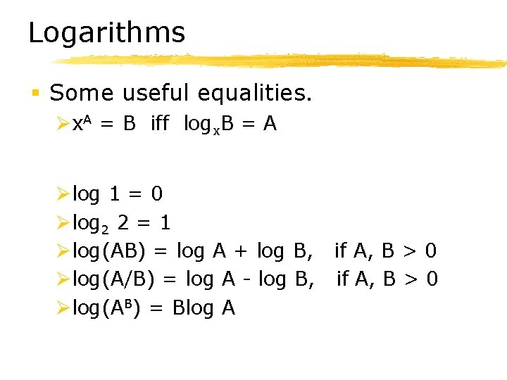
Logarithms § Some useful equalities. Øx. A = B iff logx. B = A Ølog 1 = 0 Ølog 2 2 = 1 Ølog(AB) = log A + log B, if A, B > 0 Ølog(A/B) = log A - log B, if A, B > 0 Ølog(AB) = Blog A

Upper bounds for rec. relations § Divide-and-conquer algorithms are very useful in practice. § Furthermore, they all tend to generate similar recurrence relations. § As a result, approximate upper-bound solutions are well-known for recurrence relations derived from divide-and-conquer algorithms.

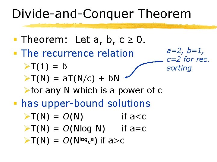
Divide-and-Conquer Theorem § Theorem: Let a, b, c 0. § The recurrence relation ØT(1) = b ØT(N) = a. T(N/c) + b. N Øfor any N which is a power of c § has upper-bound solutions ØT(N) = O(N) if a<c ØT(N) = O(Nlog N) if a=c ØT(N) = O(Nlogca) if a>c a=2, b=1, c=2 for rec. sorting

Upper-bounds § Corollary: § Dividing a problem into p pieces, each of size N/p, using only a linear amount of work, results in an O(Nlog N) algorithm.

Upper-bounds § Proof of this theorem later in the semester.

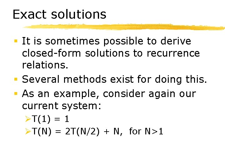
Exact solutions § It is sometimes possible to derive closed-form solutions to recurrence relations. § Several methods exist for doing this. § As an example, consider again our current system: ØT(1) = 1 ØT(N) = 2 T(N/2) + N, for N>1

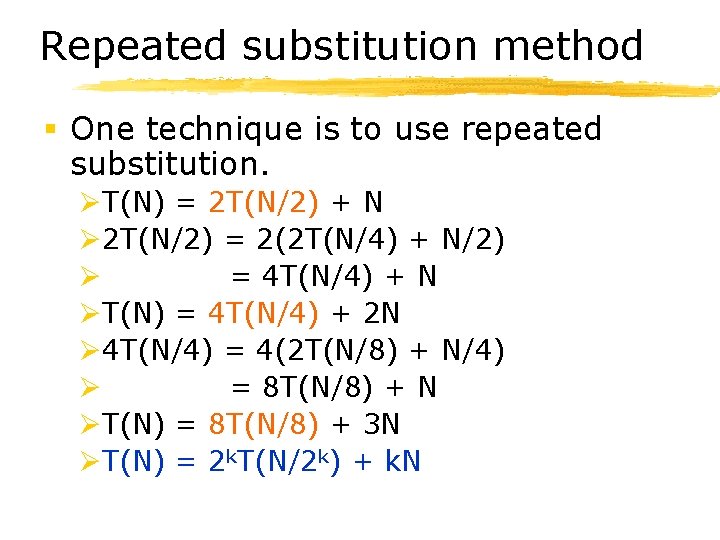
Repeated substitution method § One technique is to use repeated substitution. ØT(N) = 2 T(N/2) + N Ø 2 T(N/2) = 2(2 T(N/4) + N/2) Ø = 4 T(N/4) + N ØT(N) = 4 T(N/4) + 2 N Ø 4 T(N/4) = 4(2 T(N/8) + N/4) Ø = 8 T(N/8) + N ØT(N) = 8 T(N/8) + 3 N ØT(N) = 2 k. T(N/2 k) + k. N

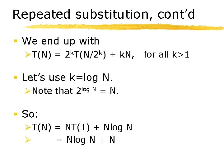
Repeated substitution, cont’d § We end up with ØT(N) = 2 k. T(N/2 k) + k. N, § Let’s use k=log N. ØNote that 2 log N = N. § So: ØT(N) = NT(1) + Nlog N Ø = Nlog N + N for all k>1

Other methods § There also other methods for solving recurrence relations. ØSee the “telescoping method” in Weiss, pp 237 -239.

Mergesort

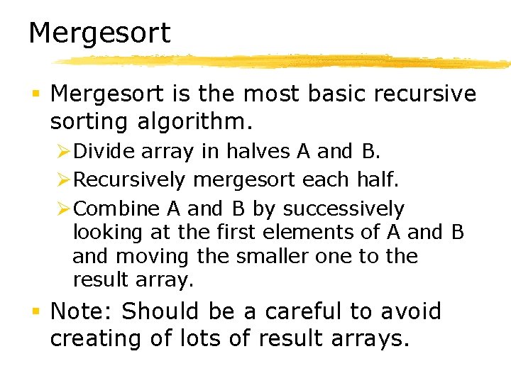
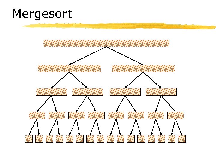
Mergesort § Mergesort is the most basic recursive sorting algorithm. ØDivide array in halves A and B. ØRecursively mergesort each half. ØCombine A and B by successively looking at the first elements of A and B and moving the smaller one to the result array. § Note: Should be a careful to avoid creating of lots of result arrays.

Mergesort

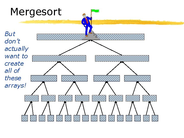
Mergesort But don’t actually want to create all of these arrays!

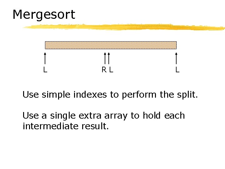
Mergesort L RL L Use simple indexes to perform the split. Use a single extra array to hold each intermediate result.

Analysis of mergesort § Mergesort generates almost exactly the same recurrence relations shown before. ØT(1) = 1 ØT(N) = 2 T(N/2) + N - 1, for N>1 § Thus, mergesort is O(Nlog N).

Quicksort

Quicksort § Quicksort was invented in 1960 by Tony Hoare. § Although it has O(N 2) worst-case performance, on average it is O(Nlog N). § More importantly, it is the fastest known comparison-based sorting algorithm in practice.

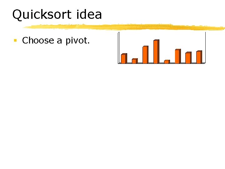
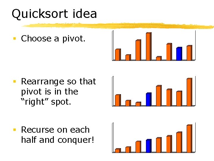
Quicksort idea § Choose a pivot.

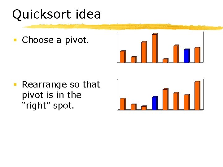
Quicksort idea § Choose a pivot. § Rearrange so that pivot is in the “right” spot.

Quicksort idea § Choose a pivot. § Rearrange so that pivot is in the “right” spot. § Recurse on each half and conquer!

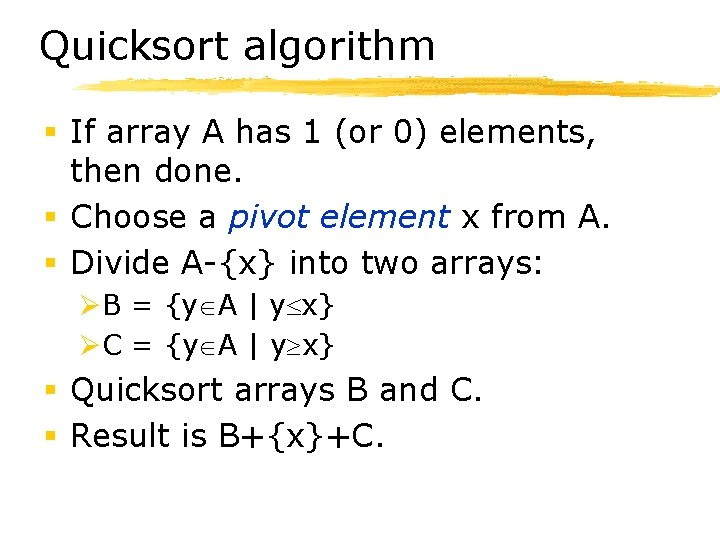
Quicksort algorithm § If array A has 1 (or 0) elements, then done. § Choose a pivot element x from A. § Divide A-{x} into two arrays: ØB = {y A | y x} ØC = {y A | y x} § Quicksort arrays B and C. § Result is B+{x}+C.

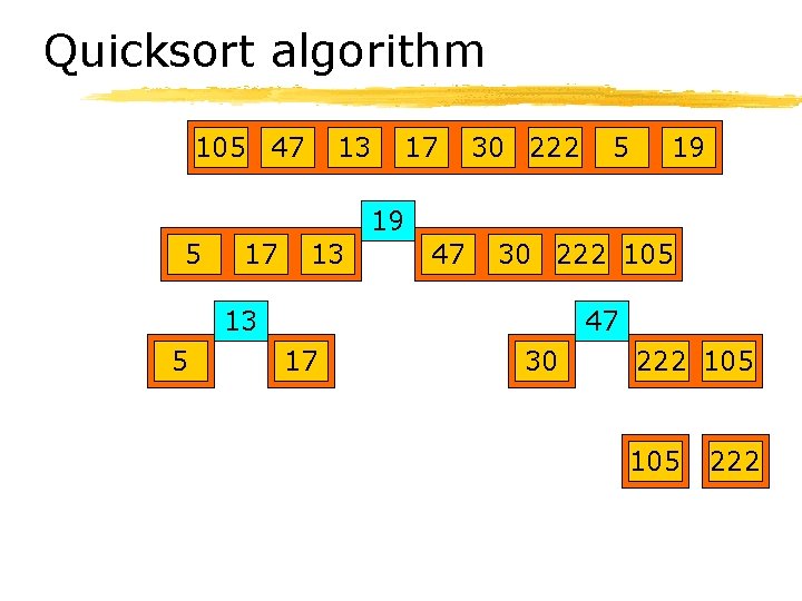
Quicksort algorithm 105 47 13 17 30 222 5 19 19 5 17 13 47 30 222 105 13 5 47 17 30 222 105 222

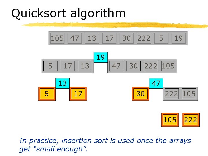
Quicksort algorithm 105 47 13 17 30 222 5 19 19 5 17 13 47 30 222 105 13 5 47 17 30 222 105 222 In practice, insertion sort is used once the arrays get “small enough”.

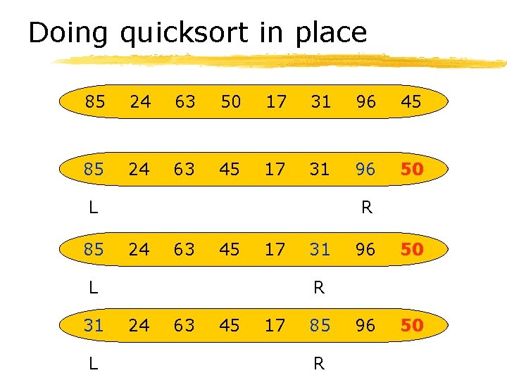
Doing quicksort in place 85 24 63 50 17 31 96 45 85 24 63 45 17 31 96 50 L 85 R 24 63 45 17 L 31 96 50 R 24 63 45 17 85 R

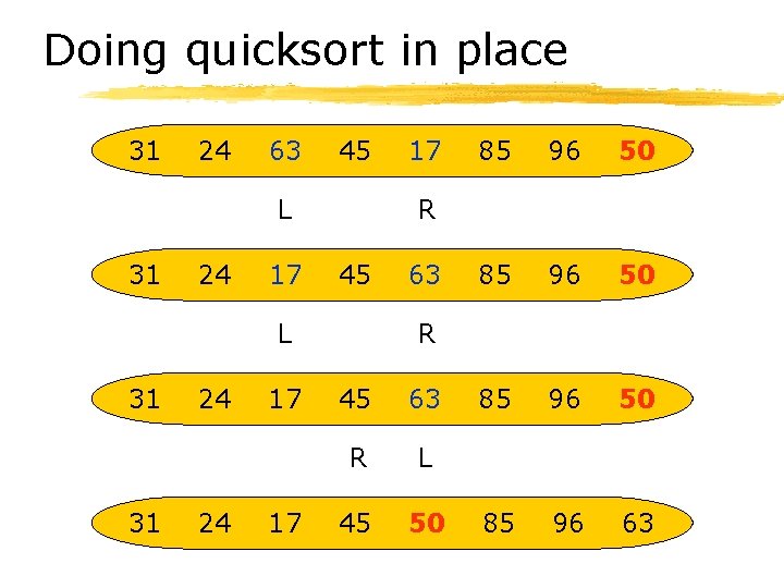
Doing quicksort in place 31 24 63 45 L 31 24 17 31 24 24 17 17 85 96 50 85 96 63 R 45 L 31 17 63 R 45 63 R L 45 50

Quicksort is fast but hard to do § Quicksort, in the early 1960’s, was famous for being incorrectly implemented many times. ØMore about invariants next time. § Quicksort is very fast in practice. ØFaster than mergesort because Quicksort can be done “in place”.

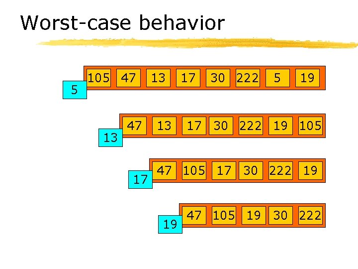
Informal analysis § If there are duplicate elements, then algorithm does not specify which subarray B or C should get them. ØIdeally, split down the middle. § Also, not specified how to choose the pivot. ØIdeally, the median value of the array, but this would be expensive to compute. § As a result, it is possible that Quicksort will show O(N 2) behavior.

Worst-case behavior 5 105 47 13 47 17 13 13 17 30 222 5 19 17 30 222 19 105 47 105 17 30 222 19 19 47 105 19 30 222

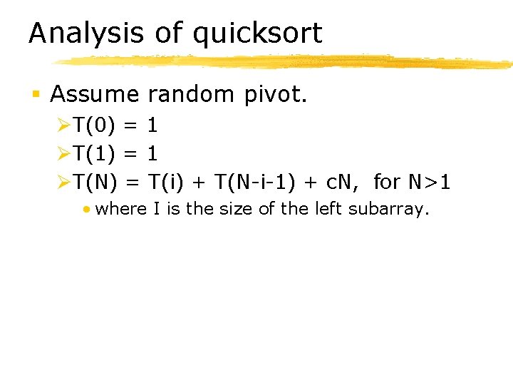
Analysis of quicksort § Assume random pivot. ØT(0) = 1 ØT(1) = 1 ØT(N) = T(i) + T(N-i-1) + c. N, for N>1 • where I is the size of the left subarray.

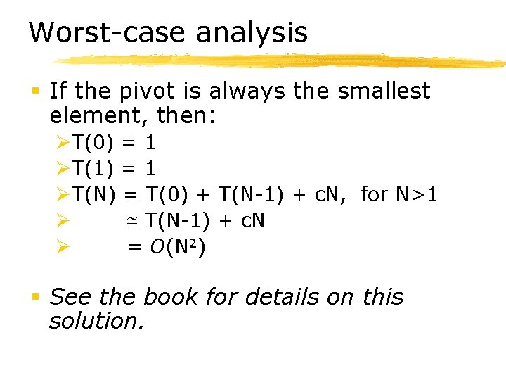
Worst-case analysis § If the pivot is always the smallest element, then: ØT(0) = 1 ØT(1) = 1 ØT(N) = T(0) + T(N-1) + c. N, for N>1 Ø T(N-1) + c. N Ø = O(N 2) § See the book for details on this solution.

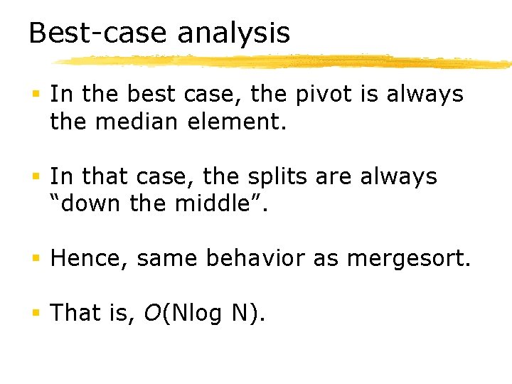
Best-case analysis § In the best case, the pivot is always the median element. § In that case, the splits are always “down the middle”. § Hence, same behavior as mergesort. § That is, O(Nlog N).

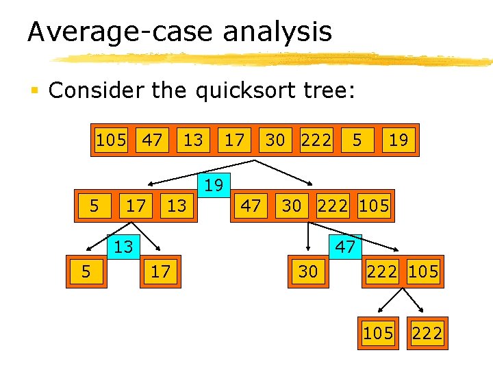
Average-case analysis § Consider the quicksort tree: 105 47 13 17 30 222 5 19 19 5 17 13 47 30 222 105 13 5 47 17 30 222 105 222

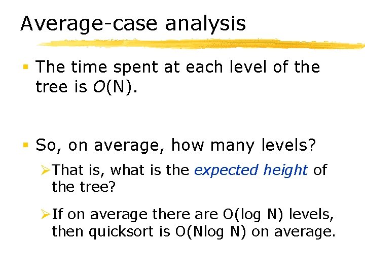
Average-case analysis § The time spent at each level of the tree is O(N). § So, on average, how many levels? ØThat is, what is the expected height of the tree? ØIf on average there are O(log N) levels, then quicksort is O(Nlog N) on average.

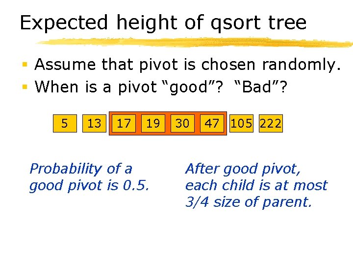
Expected height of qsort tree § Assume that pivot is chosen randomly. § When is a pivot “good”? “Bad”? 5 13 17 19 Probability of a good pivot is 0. 5. 30 47 105 222 After good pivot, each child is at most 3/4 size of parent.

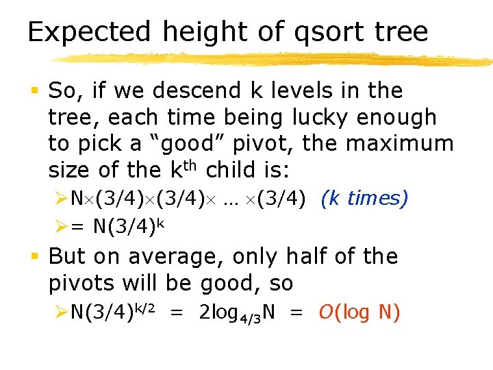
Expected height of qsort tree § So, if we descend k levels in the tree, each time being lucky enough to pick a “good” pivot, the maximum size of the kth child is: ØN (3/4) … (3/4) (k times) Ø= N(3/4)k § But on average, only half of the pivots will be good, so ØN(3/4)k/2 = 2 log 4/3 N = O(log N)

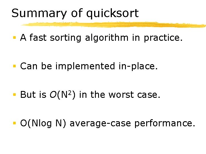
Summary of quicksort § A fast sorting algorithm in practice. § Can be implemented in-place. § But is O(N 2) in the worst case. § O(Nlog N) average-case performance.

Lower Bound for the Sorting Problem

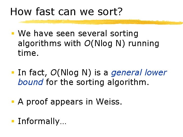
How fast can we sort? § We have seen several sorting algorithms with O(Nlog N) running time. § In fact, O(Nlog N) is a general lower bound for the sorting algorithm. § A proof appears in Weiss. § Informally…

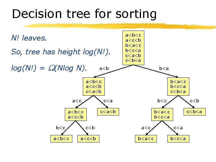
Decision tree for sorting N! leaves. So, tree has height log(N!) = (Nlog N). a<b<c a<c<b b<a<c b<c<a c<a<b c<b<a a<b<c a<c<b c<a<b b<a<c b<c<a c<b<a a<c c<a b<c c<b a<b<c a<c<b c<a<b b<a<c b<c<a c<b<a b<c a<b<c c<b a<c c<a b<a<c b<c<a

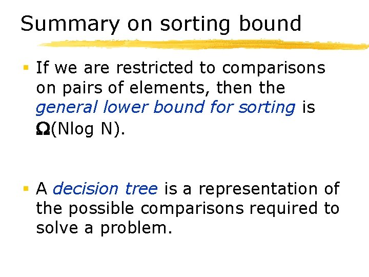
Summary on sorting bound § If we are restricted to comparisons on pairs of elements, then the general lower bound for sorting is (Nlog N). § A decision tree is a representation of the possible comparisons required to solve a problem.

Bucket Sort

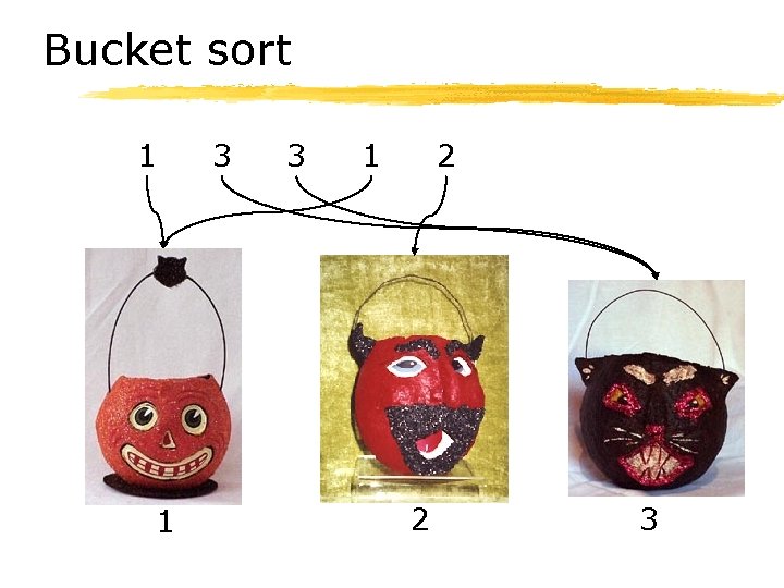
Non-comparison-based sorting § If we can use more than just comparisons of pairs of elements, we can sometimes sort more quickly. § A simple example is bucket sort. § In bucket sort, we require the additional knowledge that all elements are non-negative integers less than a specified maximum value.

Bucket sort 1 1 3 3 1 2 2 3

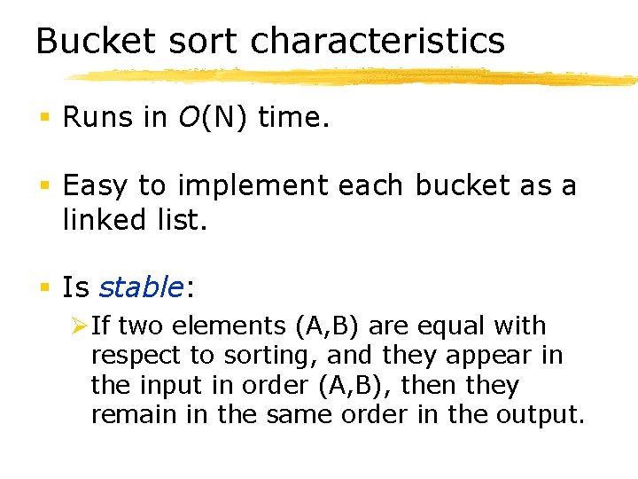
Bucket sort characteristics § Runs in O(N) time. § Easy to implement each bucket as a linked list. § Is stable: ØIf two elements (A, B) are equal with respect to sorting, and they appear in the input in order (A, B), then they remain in the same order in the output.

Radix Sort

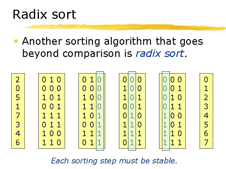
Radix sort § Another sorting algorithm that goes beyond comparison is radix sort. 2 0 5 1 7 3 4 6 0 0 1 0 1 1 1 0 0 0 1 1 0 0 1 1 1 0 1 0 0 1 1 0 1 1 0 0 0 0 0 1 1 1 1 0 0 1 1 0 1 0 1 Each sorting step must be stable. 0 1 2 3 4 5 6 7

Radix sort characteristics § Each sorting step can be performed via bucket sort, and is thus O(N). § If the numbers are all b bits long, then there are b sorting steps. § Hence, radix sort is O(b. N). § Also, radix sort can be implemented in-place (just like quicksort).

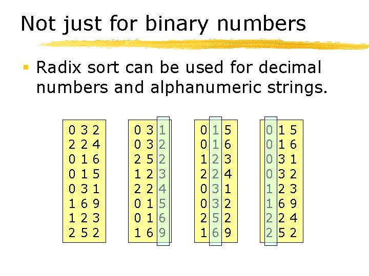
Not just for binary numbers § Radix sort can be used for decimal numbers and alphanumeric strings. 0 2 0 0 0 1 1 2 3 2 1 1 3 6 2 5 2 4 6 5 1 9 3 2 0 0 2 1 2 0 0 1 3 3 5 2 2 1 1 6 1 2 2 3 4 5 6 9 0 0 1 2 0 0 2 1 1 1 2 2 3 3 5 6 3 4 1 2 2 9 0 0 1 1 2 2 1 1 3 3 2 6 2 5 5 6 1 2 3 9 4 2