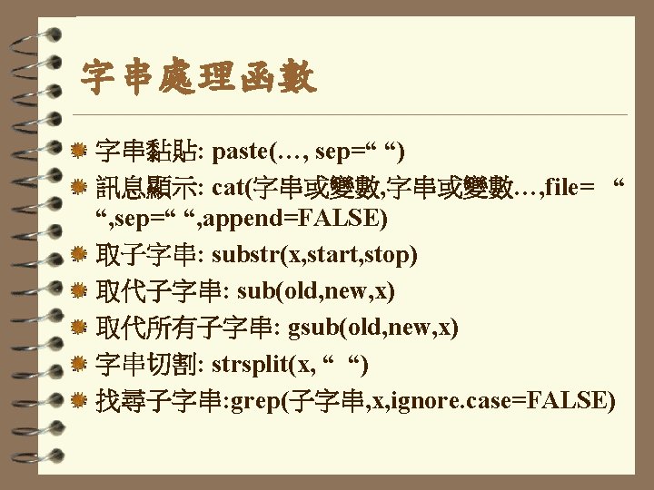
R http www rproject org mybmifunctionh w bmiwh1002


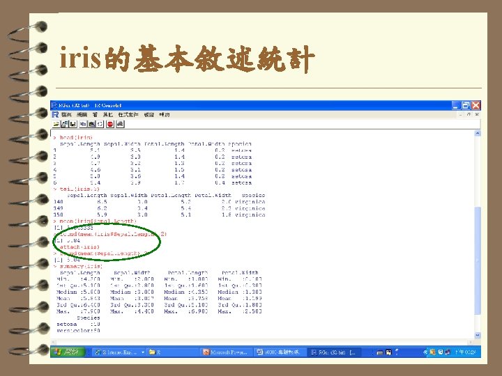
下載R軟體 http: //www. r-project. org


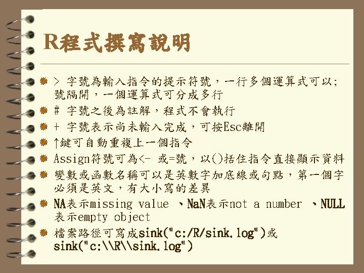
 { bmi=w/(h/100)^2 return(bmi) } 程式檔名為myfun. R")
撰寫自訂函數mybmi<-function(h, w) { bmi=w/(h/100)^2 return(bmi) } 程式檔名為myfun. R


 #設定記錄結果的檔名 sink(\"c: /R/sink. log\") summary(mydata$weight) summary(lm(mydata$height~")
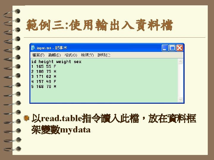
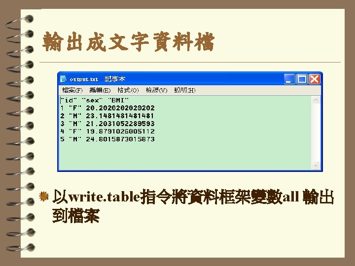
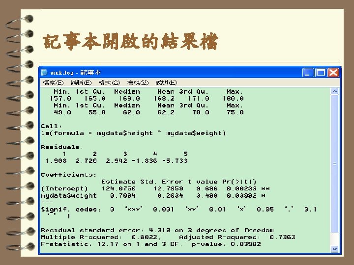
範例四: 記錄程式執行的結果 mydata=read. table("c: /r/input. txt", header= TRUE) #設定記錄結果的檔名 sink("c: /R/sink. log") summary(mydata$weight) summary(lm(mydata$height~ mydata$weight)) #以sink()結束記錄動作 sink()


 #redirect screen output to file sink(\"d:")
wdbc=read. table("d: \stella\R\wdbc. txt", header =T, sep=", ") #redirect screen output to file sink("d: \stella\R\out. txt") summary(wdbc) # descriptive statistics head(wdbc) # browse 6 records attach(wdbc) # do not need wdbc$c 1 # cat is printing function, t n are tab newline cat("c 1 mean=", round(mean(c 1), 2), "tc 1 std=", round(sd(c 1), 2), "n") cat("c 2 mean=", round(mean(c 2), "tc 2 std=", round(sd(c 2), "n") sink()


算術、比較、邏輯運算子 Arithmetic算術 Comparison比較 Logical邏輯 + addition < lesser than !x NOT - subtraction > greater than x&y AND * multiplication <= lesser than or equal to x&&y AND條件 / division >= greater than or equal to x|y OR ^ 或** power == equal x||y OR條件 %% modulo != different %/% integer division >a=c(0, 1, 0, 1) >b=c(0, 0, 1, 1) xor(x, y) exclusive OR 向量邏輯運算 >a&b或 a|b


 、 FALSE (F) Integer—整數 Double—又稱real或 numeric Complex—複數 3+2 i或寫成 x= complex( real=3,")
R的資料屬性 Logical—邏輯TRUE(T) 、 FALSE (F) Integer—整數 Double—又稱real或 numeric Complex—複數 3+2 i或寫成 x= complex( real=3, imaginary=2) Character—文字字串(character或string) name=“John” Raw—二進位資料


 sink(\"d: \stella\R\out. txt\") attach(wdbc) # do")
使用迴圈 wdbc=read. table("d: \stella\R\wdbc. txt", header=T, sep=", ") sink("d: \stella\R\out. txt") attach(wdbc) # do not need wdbc$c 1 for (i in 3: 32) { cat("c", i-2, "mean=", round(mean(wdbc[, i]), 2), "tc 1 std=", round(sd(wdbc[ , i]), 2), "n") } sink()


")
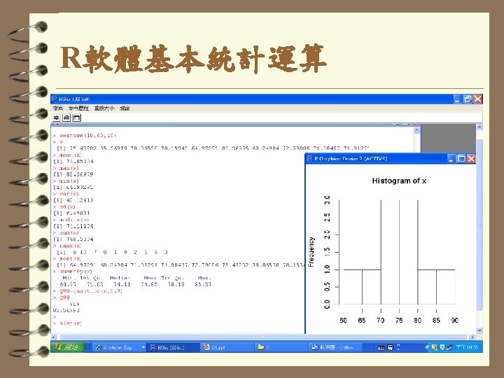
安裝R套件car 或直接 >install. packages(“car”)

")
讀取Excel檔(readxl套件)


 ifelse(邏輯判斷式, TRUE傳回值, FALSE傳回值) >newgroup=ifelse(income>=60000, ”RICH”, ”POOR”)")
重新編碼(邏輯判斷式和ifelse函數) ifelse(邏輯判斷式, TRUE傳回值, FALSE傳回值) >newgroup=ifelse(income>=60000, ”RICH”, ”POOR”)


![使用指標篩選資料 列的篩選 iris 2=iris[10: 12, ] iris 2=iris[-(10: 12), ] 欄的篩選 iris 2=iris[, 5]或iris[,](http://slidetodoc.com/presentation_image_h2/8a5ce416462d34ff475d01afee0ae9e2/image-69.jpg "使用指標篩選資料 列的篩選 iris 2=iris[10: 12, ] iris 2=iris[-(10: 12), ] 欄的篩選 iris 2=iris[, 5]或iris[,")
使用指標篩選資料 列的篩選 iris 2=iris[10: 12, ] iris 2=iris[-(10: 12), ] 欄的篩選 iris 2=iris[, 5]或iris[, ”Species”] iris 2=iris[, -5]或iris[, 1: 4] 欄列的篩選 iris 2=iris[51: 100, c(1, 2, 5)] iris 2=iris[iris$Species==“setosa, ]
![sample函數和邏輯值篩選資料 *隨機取樣 抽出不放回 *間隔取樣 每 10筆取 1 >babies[ seq(1, nrow(babies), 10), ] or >babies[as.](http://slidetodoc.com/presentation_image_h2/8a5ce416462d34ff475d01afee0ae9e2/image-70.jpg "sample函數和邏輯值篩選資料 *隨機取樣 抽出不放回 *間隔取樣 每 10筆取 1 >babies[ seq(1, nrow(babies), 10), ] or >babies[as.")
sample函數和邏輯值篩選資料 *隨機取樣 抽出不放回 *間隔取樣 每 10筆取 1 >babies[ seq(1, nrow(babies), 10), ] or >babies[as. numeric(rownames(babies) )%% 10==0, ]


![資料格式轉換(long-wide format) #stack and unstack (chicken=read. table("d: \stella\R\test. csv", sep=", ", header=T)) chicken=chicken[, -1]](http://slidetodoc.com/presentation_image_h2/8a5ce416462d34ff475d01afee0ae9e2/image-76.jpg "資料格式轉換(long-wide format) #stack and unstack (chicken=read. table(\"d: \stella\R\test. csv\", sep=\", \", header=T)) chicken=chicken[, -1]")
資料格式轉換(long-wide format) #stack and unstack (chicken=read. table("d: \stella\R\test. csv", sep=", ", header=T)) chicken=chicken[, -1] (chicken 2=stack(chicken)) #names(chicken 2)=c("weight", "feed") (chicken 3=unstack(chicken 2)) #reshape long and wide format chicken=read. table("d: \stella\R\test. csv", sep=", ", header=T) chicklong=reshape(chicken, direction="long", varying=list(c("R ation 1", "Ration 2", "Ration 3")), v. names="ration", idvar="id") chicklong chickwide=reshape(chicklong, direction="wide", idvar="id") chickwide

stack函數

unstack函數

reshape函數

")
綜合應用: 水平合併或取聯集 # method 1 : horizontal merge test=read. table("D: \stella\R\input 3. txt", header=T) t 0=test[, 1: 4] t 1=test[grep("tea", test$item 1, ignore. case=FALSE), c(1, 5)] t 2=test[grep("tea", test$item 2, ignore. case=FALSE), c(1, 6)] tt=merge(t 1, t 2, by="id", all=T) (hall=merge(t 0, tt, by="id", all. tt=T)) #method 2 : horizontal merge l 1=grep("tea", test[, 5]) l 2=grep("tea", test[, 6]) t=test[union(l 1, l 2) , ] t[order(t$id), ]

練習: 有遺漏� 的babies資料 檔 資料的筆數計有1236筆,共有7個欄位(bwt:嬰 兒體重, gestation:懷孕日數, parity:胎序, 懷孕過幾胎, age:母親年齡, height :母親身 高, weight :母親體重, smoke:母親抽煙與否 , 1表抽煙 0表不抽煙) summary(babies) nrow(babies) mean(babies$gestation, rm. na=T) babies[babies$age<18 & is. na(babies$age), ] babies=na. exclude(babies)
 attach(wdbc) for (i in 3:")
練習: wdbc分組平均數 wdbc=read. table("d: \stella\wdbc. txt", header=T, sep=", ") attach(wdbc) for (i in 3: 32) { cat(paste(“c”, i-2, sep=“”), “total mean=”, round(mean(wdbc[, i]), 4), "n") cat(“B mean=”, round(mean(wdbc[diagnosis=="B", i]), 4), "n") cat(“M mean=”, round(mean(wdbc[diagnosis=="M", i]), 4), "n") }

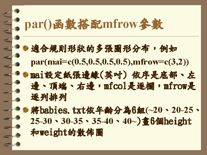
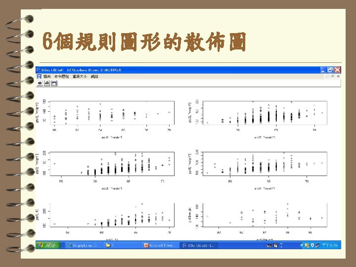
 grp 1=subset(babies, age<20) grp 2=subset(babies, age>=20 & age<25)")
多張規則圖形的程式碼 babies=read. table(“d: /R/babies. txt”, header=T) grp 1=subset(babies, age<20) grp 2=subset(babies, age>=20 & age<25) grp 3=subset(babies, age>=25 & age<30) grp 4=subset(babies, age>=30 & age<35) grp 5=subset(babies, age>=35 & age<40) grp 6=subset(babies, age>=40) #oldpar=par() par(mai=c(0. 5, 0. 5), mfrow=c(3, 2)) #by rows plot(grp 1[, "height"], grp 1[, "weight"]) #plot(x, y) x y are vectors plot(grp 2[, "height"], grp 2[, "weight"]) plot(grp 3[, "height"], grp 3[, "weight"]) plot(grp 4[, "height"], grp 4[, "weight"]) plot(grp 5[, 5], grp 5[, 6]) plot(grp 6$height, grp 6$weight) #par(oldpar)
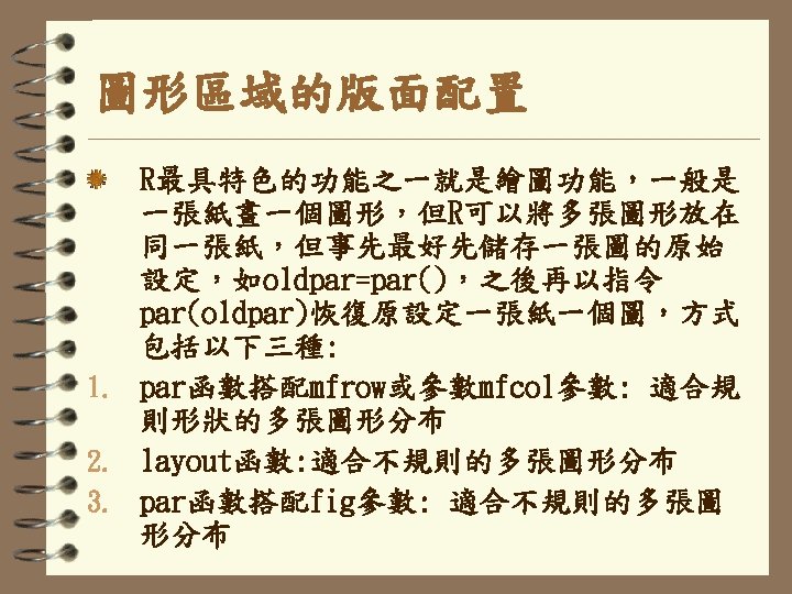
 M是圖形分佈的矩陣,widths、 heights各是設定M矩陣長、寬 的比例,其基準點是左下角 上圖的指令為 2 x 2矩陣 layout(matrix(c(1, 1,")
layout函數: 不規則的多個圖形 layout(M, widths, heights) M是圖形分佈的矩陣,widths、 heights各是設定M矩陣長、寬 的比例,其基準點是左下角 上圖的指令為 2 x 2矩陣 layout(matrix(c(1, 1, 2, 3), 2, 2, byrow=T)) 下圖的指令為 2 x 2矩陣 layout(matrix(c(2, 0, 1, 3), 2, 2, byrow=T), widths=c(3, 1), heights=c(1, 3)) 1 2 3 2 1 3
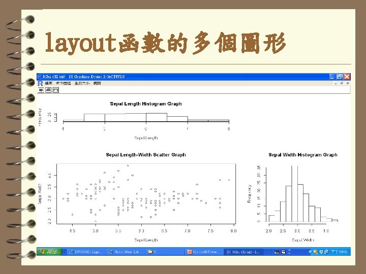
 layout(matrix(c(2, 0, 1, 3), 2, 2, byrow=T), widths=c(2, 1), heights=c(1, 2)) plot(Sepal.")
layout函數的程式碼 attach(iris) layout(matrix(c(2, 0, 1, 3), 2, 2, byrow=T), widths=c(2, 1), heights=c(1, 2)) plot(Sepal. Length, Sepal. Width, main="Se pal Length-Width Scatter Graph") hist(Sepal. Length, main="Sepal Length Histogram Graph") hist(Sepal. Width, main="Sepal Width Histogram Graph")
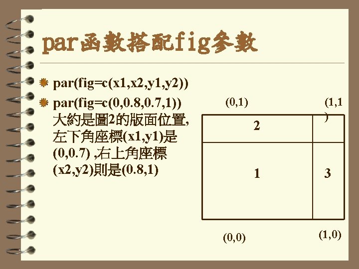
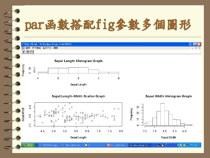
 par(fig=c(0, 0. 6, 0, 0. 6), new=TRUE) plot(Sepal. Length, Sepal. Width, main=\"Sepal")
par函數搭配fig參數程式碼 attach(iris) par(fig=c(0, 0. 6, 0, 0. 6), new=TRUE) plot(Sepal. Length, Sepal. Width, main="Sepal Length-Width Scatter Graph") par(fig=c(0, 0. 6, 1), new=TRUE) hist(Sepal. Length, main="Sepal Length Histogram Graph") par(fig=c(0. 6, 1, 0, 0. 6), new=TRUE) hist(Sepal. Width, main="Sepal Width Histogram Graph")

 >plot(Species) >plot(Sepal. Length) >plot(iris)或 pairs(iris) >plot(Species, Sepal. Length) >plot(~Sepal.")
plot散佈圖、長條圖、盒狀圖 >plot(Sepal. Length, Sepal. Width) >plot(Species) >plot(Sepal. Length) >plot(iris)或 pairs(iris) >plot(Species, Sepal. Length) >plot(~Sepal. Length+ Petal. Length+Petal. Width)
, -4, 4) curve(x^2 -4*x+3, -4, 4, lty=2, add=T)")
curve 函數曲線 curve(sin(x), -4, 4) curve(x^2 -4*x+3, -4, 4, lty=2, add=T)
")
pair矩陣圖 >pair(iris)
 > coplot(Sepal. Length~Petal. Length | Species)")
coplot條件散佈圖(加 , rows=1) > coplot(Sepal. Length~Petal. Length | Species)
 qqnorm(Sepal. Length)+ qqline(Sepal. Length)最佳線")
常態機率圖qqnorm qqline、qqplot(Sepal. Length, Sepal. Width ) qqnorm(Sepal. Length)+ qqline(Sepal. Length)最佳線
 hist(Sepal. Length, nclass=8)")
直方圖hist(Sepal. Length, breaks=4: 8) hist(Sepal. Length, nclass=8)
 labels=c(\"乳癌\", \"支氣管癌\", \"結腸癌\", \"卵巢癌 \", \"胃癌\") barplot(cancers,")
bar plot長條圖 cancers=c(11, 16, 17, 6, 12) labels=c("乳癌", "支氣管癌", "結腸癌", "卵巢癌 ", "胃癌") barplot(cancers, names=labels) barplot(cancers, names=labels, horiz=T) barplot(cancers, names=labels, col=c(1, 2, 3, 4, 5), density=10) barplot(cancers, names=labels, col=c(1, 2, 3, 4, 5), density=40)

barplot長條圖
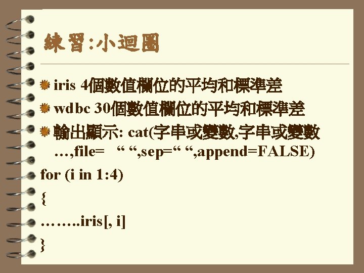
![boxplot盒狀圖 boxplot(iris[, 1], xlab="SLen", main="(F 1)") boxplot(iris[, 1: 4], main="(F 2)") boxplot(iris[, 1: 4],](http://slidetodoc.com/presentation_image_h2/8a5ce416462d34ff475d01afee0ae9e2/image-104.jpg "boxplot盒狀圖 boxplot(iris[, 1], xlab=\"SLen\", main=\"(F 1)\") boxplot(iris[, 1: 4], main=\"(F 2)\") boxplot(iris[, 1: 4],")
boxplot盒狀圖 boxplot(iris[, 1], xlab="SLen", main="(F 1)") boxplot(iris[, 1: 4], main="(F 2)") boxplot(iris[, 1: 4], main="(F 3)", names=c("Slen", "Swid", "Plen", "Pwid")) boxplot(iris[, 1: 4], main="(F 4)", horizontal=T) boxplot(iris[, 4]~iris[, 5], main="(F 5)", xlab="flow er class", ylab="Slen") boxplot(Sepal. Length~Species, data=iris, main=" (F 6)", xlab="flower class", ylab="Slen“ , col=c(2, 3, 4))

boxplot盒狀圖
")
Pie圓餅圖 sales=c(0. 12, 0. 3 , 0. 26, 0. 16, 0. 04, 0. 12) snames=c("電 腦", "廚具", "家 電", "傢俱", "其 他", "服飾") pie(sales, label= snames)
: 畫出地圖效果的等高線圖 image(x, y, z): 類似於contour,但可畫出色彩 persp(x,")
3 D繪圖contour 、 image 、persp contour(x, y, z): 畫出地圖效果的等高線圖 image(x, y, z): 類似於contour,但可畫出色彩 persp(x, y, z, theta, phi, box=TRUE): 畫出真正 的三度空間透視圖,theta控制圖形上下旋轉角 度,phi控制圖形左右旋轉角度,box=TRUE則不 畫出框線 >demo(graphics) #展示繪圖功能 等高線圖 >filled. contour(volcano, color=terrain. col ors, plot. axes=contour(volcano, add=TRUE))
 y=x f=function(x, y){(1/(2*pi))*exp(-0. 5*(x^2+y^2))} z=outer(x,")
3 D繪圖contour 、 image 、persp x=seq(-3, 3, 0. 1) y=x f=function(x, y){(1/(2*pi))*exp(-0. 5*(x^2+y^2))} z=outer(x, y, f) #外積函數outer par(mfcol=c(2, 2)) contour(x, y, z) image(x, y, z) persp(x, y, z, theta=30, phi=30, box=F, main= "persp theta=30 phi=30")

3 D繪圖contour 、 image 、persp
 、 ylim=c(0, 30) add=TRUE #覆蓋前一張圖 axes=FALSE")
繪圖函數的共用輔助參數 main=“” 、 sub=“” 、xlab=“” 、ylab=“” xlim=c(xmin, xmax) 、 ylim=c(0, 30) add=TRUE #覆蓋前一張圖 axes=FALSE #不畫出座標軸 xaxt=“n” yaxt=“n” #不畫出座標軸格線 right=FALSE #即右邊為開放區間 < log=“x”、 log=“y”、 log=“xy” type=“p”: points only 、type=“l”: lines only type=“b”: points and lines、 type=“o”: overlap type=“s”: steps 、type=“h”: height
 >plot(x, type=“p”) >plot(x, type=“o”) >plot(x, type=“l”) >plot(x, type=“s”) >plot(x, type=“b”)")
plot圖點樣式 x=rnorm(10, 0, 1) >plot(x, type=“p”) >plot(x, type=“o”) >plot(x, type=“l”) >plot(x, type=“s”) >plot(x, type=“b”) >plot(x, type=“h”)
 score=sample(c(60: 100), 30, replace=TRUE) xp=c(160, 165, 170, 175)")
附加圖形: points、lines、text height=sample(150: 190, 30, replace=TRUE) score=sample(c(60: 100), 30, replace=TRUE) xp=c(160, 165, 170, 175) yp=c(80, 90, 80, 90) plot(height, score) points(xp, yp, col=2, pch=19) lines(xp, yp, col=3) text(xp, yp+5, col=4, label=c("P 1", "P 2", "P 3", "P 4"))
 sex=sample(c(\"M\", \"F\"), 100, replace=TRUE) race=sample(c(\"WHITE \", \"YELLOW\", \"BLACK")
附加圖形: legend、title、axis age=sample(20: 60, 100, replace=TRUE) sex=sample(c("M", "F"), 100, replace=TRUE) race=sample(c("WHITE ", "YELLOW", "BLACK "), 100, replace=TRUE) data=data. frame(age, sex, race) barplot(table(race), col= 4: 6) table(race) 28 31 41
 F 8 17 21 M 20 14 20 barplot(table(sex, race),")
附加圖形: legend、title、axis table(sex, race) F 8 17 21 M 20 14 20 barplot(table(sex, race), col =c(“pink”, “blue”), axes= FALSE, beside=TRUE) legend(0. 5, 40, c("Female", " Male"), col=c("pink", "blue "), pch=15) title(main="Race and Sex Bar Chart", sub="in 1988") axis(2, las=2) 1底部 2左邊 las=2水平數字
![也可在既有圖形加入add=T boxplot(age~race, main="Age by Race", col="yellow", boxwex= 0. 3) boxplot(age[sex== "M"]~race[sex=="M" ], col="blue", boxwex=](http://slidetodoc.com/presentation_image_h2/8a5ce416462d34ff475d01afee0ae9e2/image-115.jpg "也可在既有圖形加入add=T boxplot(age~race, main=\"Age by Race\", col=\"yellow\", boxwex= 0. 3) boxplot(age[sex== \"M\"]~race[sex==\"M\" ], col=\"blue\", boxwex=")
也可在既有圖形加入add=T boxplot(age~race, main="Age by Race", col="yellow", boxwex= 0. 3) boxplot(age[sex== "M"]~race[sex=="M" ], col="blue", boxwex= 0. 1, at= c(1. 3, 2. 3, 3. 3), add=TRUE, axes=F)
 plot(Sepal. Length, Petal. Length, xaxt=\"n\", yaxt= \"n\", xlim=c(4, 8)) axis(side=1, at=seq(4, 8,")
自訂座標軸及互動式圖形 attach(iris) plot(Sepal. Length, Petal. Length, xaxt="n", yaxt= "n", xlim=c(4, 8)) axis(side=1, at=seq(4, 8, b y=0. 5)) axis(side=2, las=2) abline(v=7, col="red") identify(Sepal. Length, P etal. Length) 按右鍵的停止功能結束
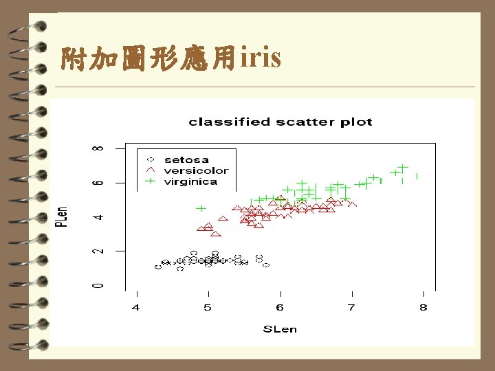
![附加圖形應用: points、 legend plot(Sepal. Length[Species=="setosa"], Petal. Len gth[Species=="setosa"], pch=1 , col="black", xlim=c(4, 8), ylim=](http://slidetodoc.com/presentation_image_h2/8a5ce416462d34ff475d01afee0ae9e2/image-117.jpg "附加圖形應用: points、 legend plot(Sepal. Length[Species==\"setosa\"], Petal. Len gth[Species==\"setosa\"], pch=1 , col=\"black\", xlim=c(4, 8), ylim=")
附加圖形應用: points、 legend plot(Sepal. Length[Species=="setosa"], Petal. Len gth[Species=="setosa"], pch=1 , col="black", xlim=c(4, 8), ylim= c(0, 8), main="classified scatter plot", xlab= "SLen", ylab= "PLen") points(Sepal. Length[Species=="virginica"], Peta l. Length[Species=="virginica"], pch=3, col="gre en") points(Sepal. Length[Species=="versicolor"], Pet al. Length[Species=="versicolor"], pch=2, col="r ed") legend(4, 8, legend=c("setosa", "versicolor", "virg inica"), col=c(1, 2, 3), pch=c(1, 2, 3))

Taiwan map
![Taiwan map library(maps) x=world. cities taiwan=x[x$country. etc=="Taiwan", ] taiwan map("world", xlim=c(120, 122), ylim=c(21. 2,](http://slidetodoc.com/presentation_image_h2/8a5ce416462d34ff475d01afee0ae9e2/image-120.jpg "Taiwan map library(maps) x=world. cities taiwan=x[x$country. etc==\"Taiwan\", ] taiwan map(\"world\", xlim=c(120, 122), ylim=c(21. 2,")
Taiwan map library(maps) x=world. cities taiwan=x[x$country. etc=="Taiwan", ] taiwan map("world", xlim=c(120, 122), ylim=c(21. 2, 25. 5), mar=c(1, 1 , 1, 1)) taiwan. city=taiwan[taiwan$name %in% c("Taipei", "Taoyuan", "Taichung", "Tainan", "Kaohsiung"), ] map. cities(taiwan. city, capital=1) map. cities(taiwan. city, label=TRUE) mpop=taiwan[taiwan$pop >1000000, ] symbols(mpop$long, mpop$lat, circle=mpop$pop, inches=0. 2, fg=2, lwd=2, add=TRUE)
![Scatterplot 3 d之一 library("scatterplot 3 d") scatterplot 3 d(iris[, 1: 3], angle=55, main="3 D](http://slidetodoc.com/presentation_image_h2/8a5ce416462d34ff475d01afee0ae9e2/image-121.jpg "Scatterplot 3 d之一 library(\"scatterplot 3 d\") scatterplot 3 d(iris[, 1: 3], angle=55, main=\"3 D")
Scatterplot 3 d之一 library("scatterplot 3 d") scatterplot 3 d(iris[, 1: 3], angle=55, main="3 D Scatter Plot", xlab = "Sepal Length (cm)", ylab = "Sepal Width (cm)", zlab = "Petal Length (cm)") scatterplot 3 d(iris[, 1: 3], pch = 16, color="steelblue")

Scatterplot 3 d之一

Scatterplot 3 d之二 #Change point shapes and colors by groups shapes = c(16, 17, 18) shapes <- shapes[as. numeric(iris$Species)] scatterplot 3 d(iris[, 1: 3], pch = shapes) colors <- c("#999999", "#E 69 F 00", "#56 B 4 E 9") colors <- colors[as. numeric(iris$Species)] scatterplot 3 d(iris[, 1: 3], pch = 16, color=colors)

Scatterplot 3 d之二
![Scatterplot 3 d之三 #Remove box and add bars scatterplot 3 d(iris[, 1: 3], pch](http://slidetodoc.com/presentation_image_h2/8a5ce416462d34ff475d01afee0ae9e2/image-125.jpg "Scatterplot 3 d之三 #Remove box and add bars scatterplot 3 d(iris[, 1: 3], pch")
Scatterplot 3 d之三 #Remove box and add bars scatterplot 3 d(iris[, 1: 3], pch = 16, color = colors, grid=TRUE, box=FALSE) scatterplot 3 d(iris[, 1: 3], pch = 16, type="h", color=colors)

Scatterplot 3 d之三

Scatterplot 3 d之四 # Custom shapes/colors legends or points label s 3 d <- scatterplot 3 d(iris[, 1: 3], pch = shapes, color=colors) legend("bottom", legend = levels(iris$Species), col = c("#999999", "#E 69 F 00", "#56 B 4 E 9"), pch = c(16, 17, 18), inset = -0. 25, xpd = TRUE, horiz = TRUE, cex=0. 5) # inset: distance between plot and legend # xpd: enable legend outside plot scatterplot 3 d(iris[, 1: 3], pch = 16, color=colors) text(s 3 d$xyz. convert(iris[, 1: 3]), labels = rownames(iris), cex= 0. 7, col = "steelblue")

Scatterplot 3 d之四
 par(mfcol=c(1, 2)) s 3 d=scatterplot 3 d(Nuts, Eggs, Milk, col.")
Scatterplot 3 d之五 oldpar=par() par(mfcol=c(1, 2)) s 3 d=scatterplot 3 d(Nuts, Eggs, Milk, col. axis="blue", col. grid="lightblue", main="scatterplot 3 d - 1", pch=16, color=as. numeric(Country)) text(s 3 d$xyz. convert(data[, c(9, 4, 5)]), labels = Country, cex= 0. 6, col = "steelblue") t 3 d=scatterplot 3 d(Red. Meat, White. Meat, Fish, col. axis="blue", col. grid="lightblue", main="scatterplot 3 d - 2", pch=16, color=as. numeric(Country)) text(t 3 d$xyz. convert(data[, c(2, 3, 6)]), labels = Country, cex= 0. 6, col = "steelblue") par(oldpar)

Scatterplot 3 d之五

plot 3 D套組說明 scatter 3 D(x, y, z, . . . , colvar = z, col = NULL, add = FALSE) text 3 D(x, y, z, labels, colvar = NULL, add = FALSE) points 3 D(x, y, z, . . . ) #scatter 3 D(…, type =“p”) lines 3 D(x, y, z, . . . ) #scatter 3 D(…, type =“l”) scatter 2 D(x, y, colvar = NULL, col = NULL, add = FALSE) text 2 D(x, y, labels, colvar = NULL, col = NULL, add = FALSE)

plot 3 D套組說明 x, y, z: vectors of point coordinates colvar: a variable used for coloring by z , unless colvar = NULL col: color palette used for coloring colvar variable labels: the text to be written add: logical. If TRUE, then the points will be added to the current plot. If FALSE a new plot is started …: additional persp arguments including xlim, ylim, zlim, xlab, ylab, zlab, main, sub, r, d, scale, expand, box, axes, nticks, tictype.
 attach(iris) x=Sepal. Length; y=Petal. Length; z=Sepal. Width oldpar=par()")
scatter 3 D之一 library(plot 3 D) attach(iris) x=Sepal. Length; y=Petal. Length; z=Sepal. Width oldpar=par() par(mfcol=c(1, 2)) #By default, the points are colored automatically using the variable Z scatter 3 D(x, y, z, clab = c("Sepal", "Width (cm)")) scatter 3 D(x, y, z, colvar = NULL, col = "blue", pch = 19, cex = 0. 5) par(oldpar)

scatter 3 D之一

scatter 3 D之二 #title and axis labels scatter 3 D(x, y, z, phi = 0, bty = "g", pch = 20, cex = 2, ticktype = "detailed", main = "Iris data", xlab = "Sepal. Length", ylab ="Petal. Length", zlab = "Sepal. Width") # Create a scatter plot and text scatter 3 D(x, y, z, phi = 0, bty = "g", pch = 20, cex = 0. 5) text 3 D(x, y, z, labels = rownames(iris), add = TRUE, colkey = FALSE, cex = 0. 5)

scatter 3 D之二
 attach(data) scatter 3 D(Nuts, Fr. Veg,")
scatter 3 D之三 data=read. table("d: \stella\R\protein. txt", header=T) attach(data) scatter 3 D(Nuts, Fr. Veg, Fish, phi = 0, bty = "g", colvar = NULL, col = "red", pch = 16, cex = 0. 5, main = "6 variables (red & blue)", xlab = "Nuts & Eggs", ylab ="Fr. Veg & White. Meat", zlab = "Fish & Rea. Meat") text 3 D(Nuts, Fr. Veg, Fish, labels =rownames(data), add = TRUE, colkey = FALSE, cex = 0. 5) scatter 3 D(Eggs, White. Meat, Red. Meat, colvar = NULL, col = "blue", pch = 19, cex = 0. 5, add=T) text 3 D(Eggs, White. Meat, Red. Meat, labels = rownames(data), add=TRUE, colkey = FALSE, cex = 0. 5)

scatter 3 D之三

scatter 3 D之四 # 4 D and choose suitable ranges with(USArrests, text 3 D(Murder, Assault, Rape, labels = rownames(USArrests), colvar = Urban. Pop, col = gg. col(100), theta = 60, phi = 20, xlab = "Murder", ylab = "Assault", zlab = "Rape", main = "USA arrests", cex = 0. 6, bty = "g", ticktype = "detailed", d = 2, clab = c("Urban", "Pop"), adj = 0. 5, font = 2)) with(USArrests, scatter 3 D(Murder, Assault, Rape - 1, colvar = Urban. Pop, col = gg. col(100), type = "h", pch = ". ", add = TRUE)) plotdev(xlim = c(0, 10), ylim = c(40, 150), zlim = c(7, 25))

scatter 3 D之四
 library(lattice) plot(xyplot(long~lat| cut(depth, 2))) Magnitude=equal. count(mag, 6) plot(cloud(depth~lat* long| Magnitude, panel. aspect=0.")
Lattice套組 attach(quakes) library(lattice) plot(xyplot(long~lat| cut(depth, 2))) Magnitude=equal. count(mag, 6) plot(cloud(depth~lat* long| Magnitude, panel. aspect=0. 9)) plot(cloud(depth~lat* long| cut(mag, 4), panel. aspect=0. 9)) summary(Deep) plot(lat~long, pch='+') symbols(long, lat, circles=depth, inches=0. 5, add=T)

Lattice兩格

Lattice六格

Lattice四格

Lattice四格

Bubble plot
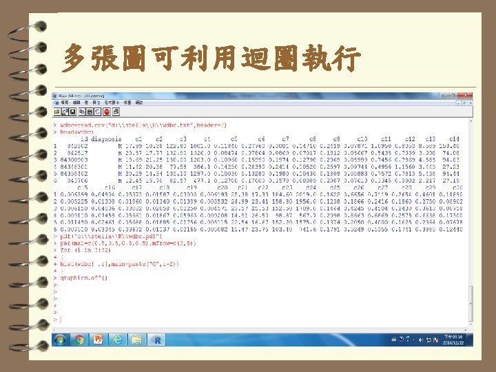
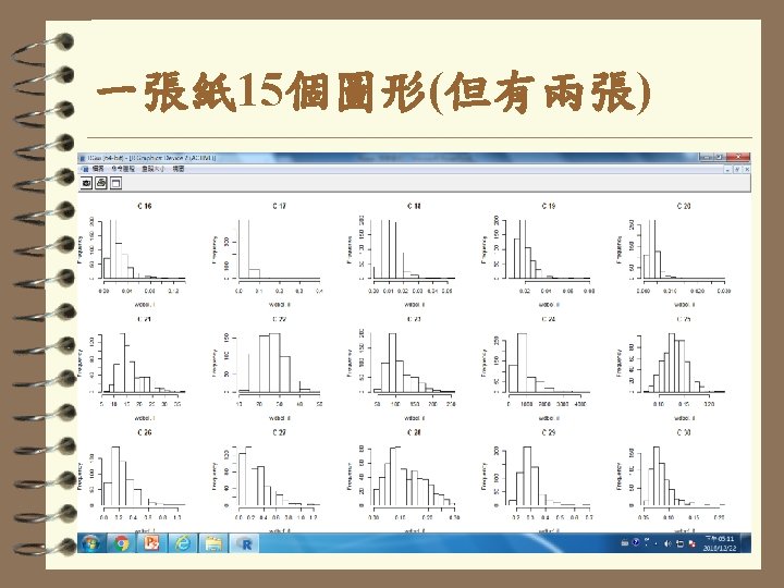
 head(wdbc) pdf(\"d: \stella\R\wdbc. pdf\") par(mai=c(0. 5, 0.")
兩張紙 30個圖形輸出到pdf檔 wdbc=read. csv(“d: \stella\R\wdbc. txt”, header=T) head(wdbc) pdf("d: \stella\R\wdbc. pdf") par(mai=c(0. 5, 0. 5), mfrow=c(3, 5)) for (i in 3: 32) { hist(wdbc[ , i], main=paste("C", i-2)) } graphics. off()
 # method 1: all files of one directory (dir=list. files(\"d: /stella/R/baby\", full. name=TRUE))")
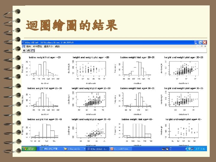
迴圈繪圖(多個檔在同一目錄) # method 1: all files of one directory (dir=list. files("d: /stella/R/baby", full. name=TRUE)) # infile=dir[grep(“. txt”, dir)] par(mai=c(0. 5, 0. 5), mfrow=c(3, 4)) lbl=c("~20", "20~25", "25~30", "30~35", "35~40", "40~") for (i in 1: length(dir)) { file 0=dir[i]; data=read. table(file=file 0, header=T) hist(data$bwt, main=paste("babies weight hist age=", lbl[i])) plot(data$height, data$weight, main=paste("height and weight plot age=", lbl[i])) }

 #method 2: seqential file names利用循序檔名 pdf(\"d: \stella\R\baby\babies. pdf\") # , family=“GB 1” par(mai=c(0.")
迴圈繪圖(利用循序的檔名) #method 2: seqential file names利用循序檔名 pdf("d: \stella\R\baby\babies. pdf") # , family=“GB 1” par(mai=c(0. 5, 0. 5), mfrow=c(3, 2)) lbl=c("~20", "20~25", "25~30", "30~35", "35~40", "40~") for (i in 1: 6) { fn=paste("d: \stella\R\baby", i, ". txt", sep=""); data=read. table(file=fn, header=T) hist(data$bwt, main=paste("babies weight hist age=", lbl[i])) plot(data$height, data$weight, main=paste("height and weight plot age=", lbl[i])) } graphics. off() # or dev. off()
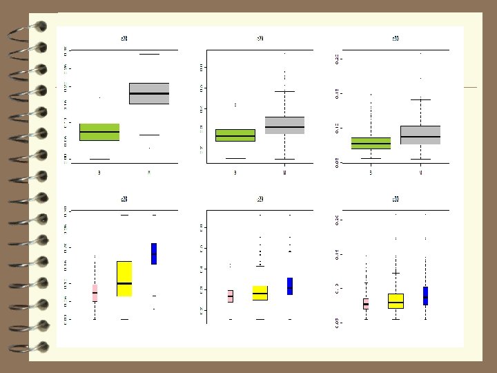
 par(mai=c(0. 5, 0. 5), mfcol=c(2, 3)) for (i in")
練習: wdbc盒狀圖 pdf("d: \stella\output. pdf") par(mai=c(0. 5, 0. 5), mfcol=c(2, 3)) for (i in 3: 32) { boxplot(wdbc[, i]~wdbc[, 2], main=paste("c", i 2, sep=""), col=c("yellowgreen", "gray")) boxplot(wdbc[, i], main=paste("c", i-2, sep=""), col="yellow", boxwex=0. 3) boxplot(wdbc[diagnosis==“M”, i], col=“blue”, boxwex= 0. 1, c(1. 3), add=TRUE, axes=F) boxplot(wdbc[diagnosis==“B”, i], col=“pink”, boxwex= 0. 1, c(0. 7), add=TRUE, axes=F) } graphics. off() at=
- Slides: 155