Quantum Spectrum Testing Ryan ODonnell John Wright Carnegie

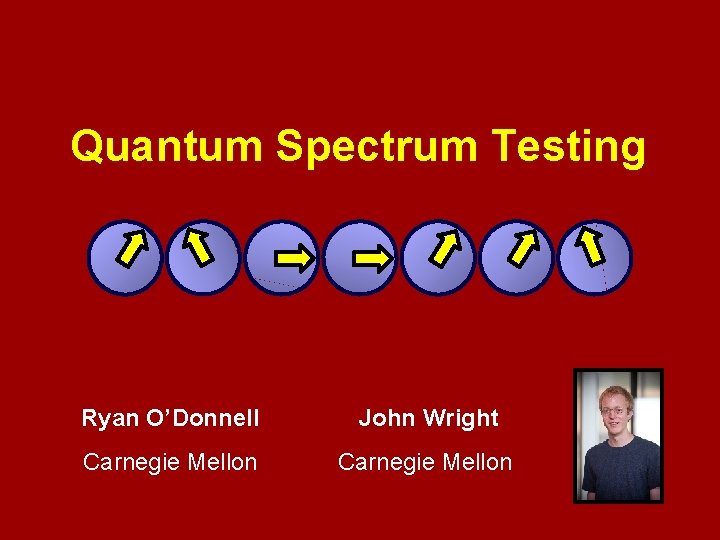
Quantum Spectrum Testing Ryan O’Donnell John Wright Carnegie Mellon

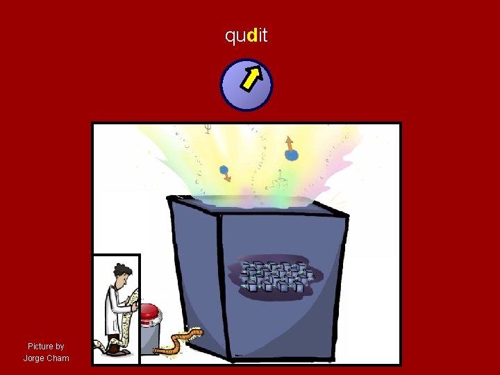
qudit Picture by Jorge Cham

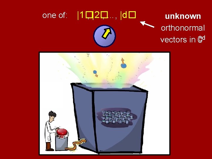
one of: |1� , |2� , …, |d� unknown orthonormal vectors in ℂd

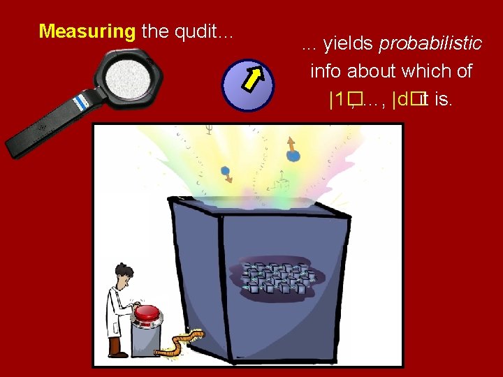
Measuring the qudit… . . . yields probabilistic info about which of |1� , …, |d�it is.

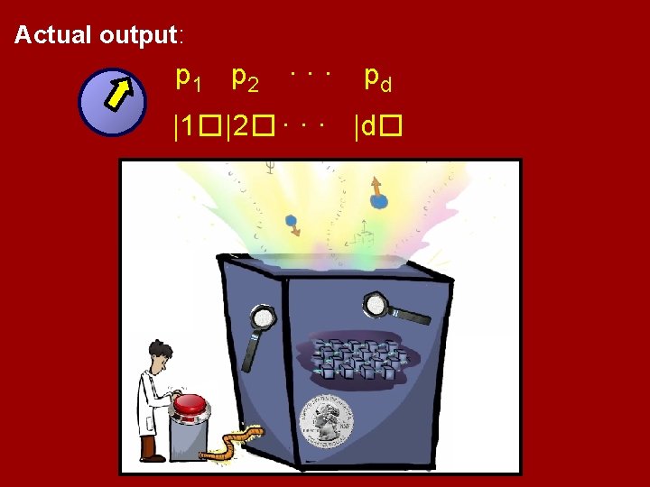
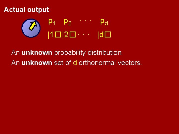
Actual output: p 1 p 2 · · · pd |1�|2� · · · |d�

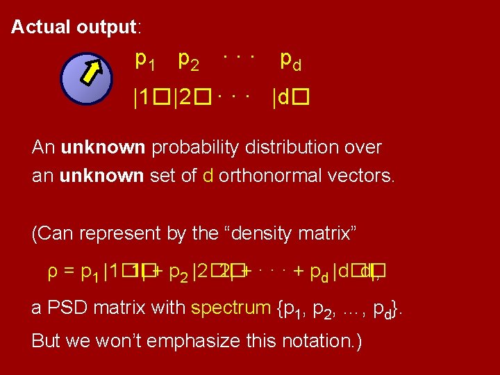
Actual output: p 1 p 2 · · · pd |1�|2� · · · |d� An unknown probability distribution over an unknown set of d orthonormal vectors. (Can represent by the “density matrix” ρ = p 1 |1�� 1| + p 2 |2�� 2| + · · · + pd |d�� d|, a PSD matrix with spectrum {p 1, p 2, …, pd}. But we won’t emphasize this notation. )

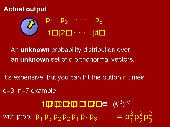
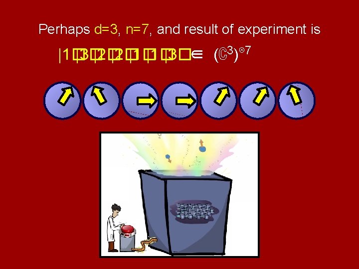
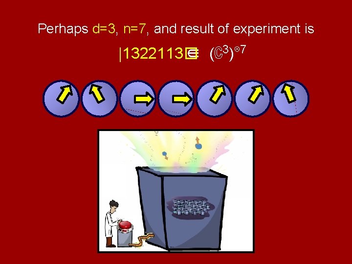
Actual output: p 1 p 2 · · · pd |1�|2� · · · |d� An unknown probability distribution over an unknown set of d orthonormal vectors. It’s expensive, but you can hit the button n times. d=3, n=7 example: |1� |3� |2� |1� |3�∈ (ℂ3)⊗ 7 with prob. p 1 p 3 p 2 p 1 p 3

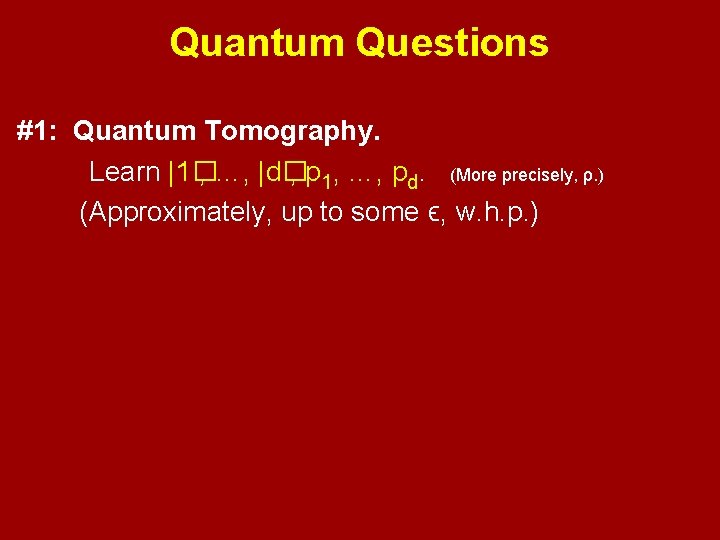
Quantum Questions #1: Quantum Tomography. Learn |1� , …, |d� , p 1, …, pd. (More precisely, ρ. ) (Approximately, up to some ϵ, w. h. p. )

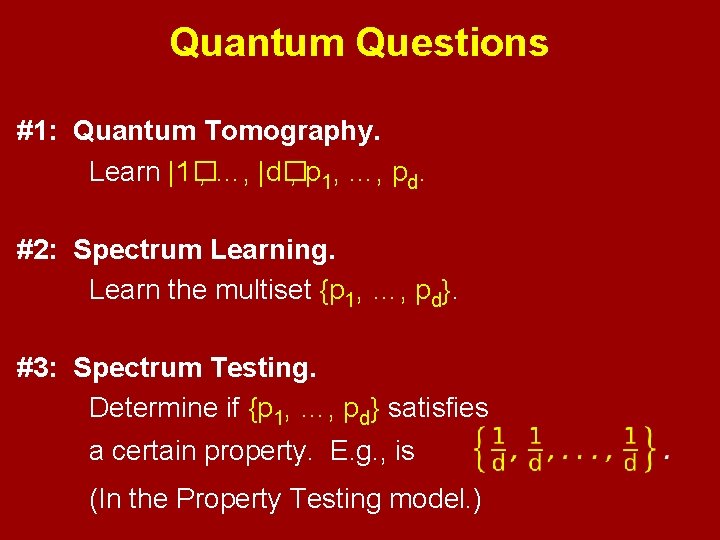
Quantum Questions #1: Quantum Tomography. Learn |1� , …, |d� , p 1, …, pd. #2: Spectrum Learning. Learn the multiset {p 1, …, pd}. (Approximately, up to some ϵ, w. h. p. )

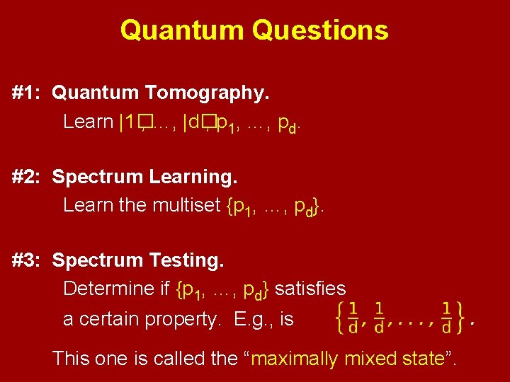
Quantum Questions #1: Quantum Tomography. Learn |1� , …, |d� , p 1, …, pd. #2: Spectrum Learning. Learn the multiset {p 1, …, pd}. #3: Spectrum Testing. Determine if {p 1, …, pd} satisfies a certain property. E. g. , is (In the Property Testing model. )

Quantum Questions #1: Quantum Tomography. Learn |1� , …, |d� , p 1, …, pd. #2: Spectrum Learning. Learn the multiset {p 1, …, pd}. #3: Spectrum Testing. Determine if {p 1, …, pd} satisfies a certain property. E. g. , is This one is called the “maximally mixed state”.

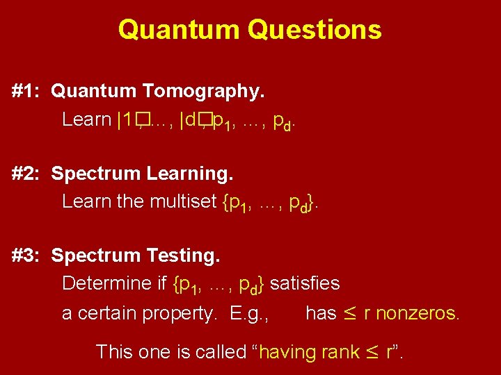
Quantum Questions #1: Quantum Tomography. Learn |1� , …, |d� , p 1, …, pd. #2: Spectrum Learning. Learn the multiset {p 1, …, pd}. #3: Spectrum Testing. Determine if {p 1, …, pd} satisfies a certain property. E. g. , has ≤ r nonzeros. This one is called “having rank ≤ r”.

Actual output: p 1 p 2 · · · pd |1�|2� · · · |d� An unknown probability distribution. An unknown set of d orthonormal vectors.

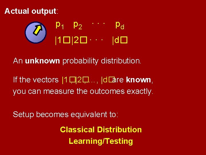
Actual output: p 1 p 2 · · · pd |1�|2� · · · |d� An unknown probability distribution. If the vectors |1� , |2� , …, |d�are known, you can measure the outcomes exactly. Setup becomes equivalent to: Classical Distribution Learning/Testing

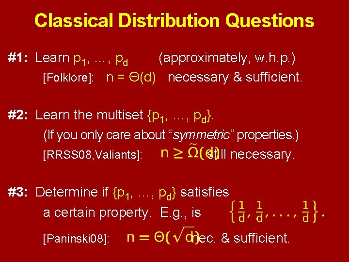
Classical Distribution Questions #1: Learn p 1, …, pd (approximately, w. h. p. ) [Folklore]: n = Θ(d) necessary & sufficient. #2: Learn the multiset {p 1, …, pd}. (If you only care about “symmetric” properties. ) [RRSS 08, Valiants]: still necessary. #3: Determine if {p 1, …, pd} satisfies a certain property. E. g. , is [Paninski 08]: nec. & sufficient.

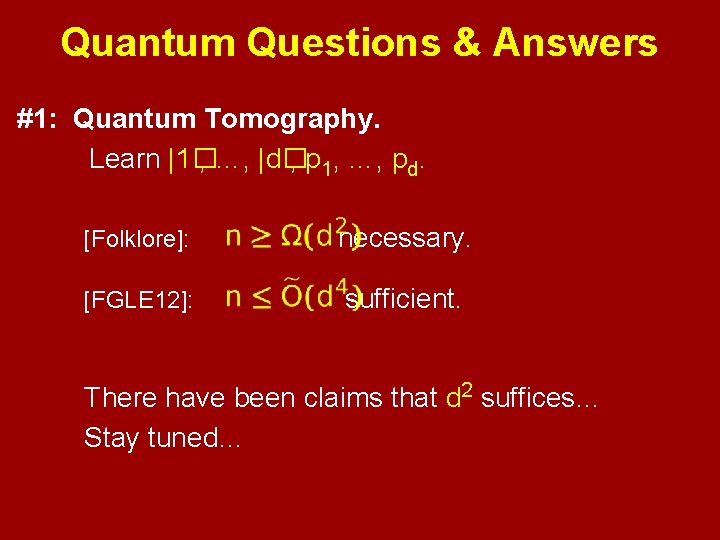
Quantum Questions & Answers #1: Quantum Tomography. Learn |1� , …, |d� , p 1, …, pd. [Folklore]: necessary. [FGLE 12]: sufficient. There have been claims that d 2 suffices… Stay tuned…

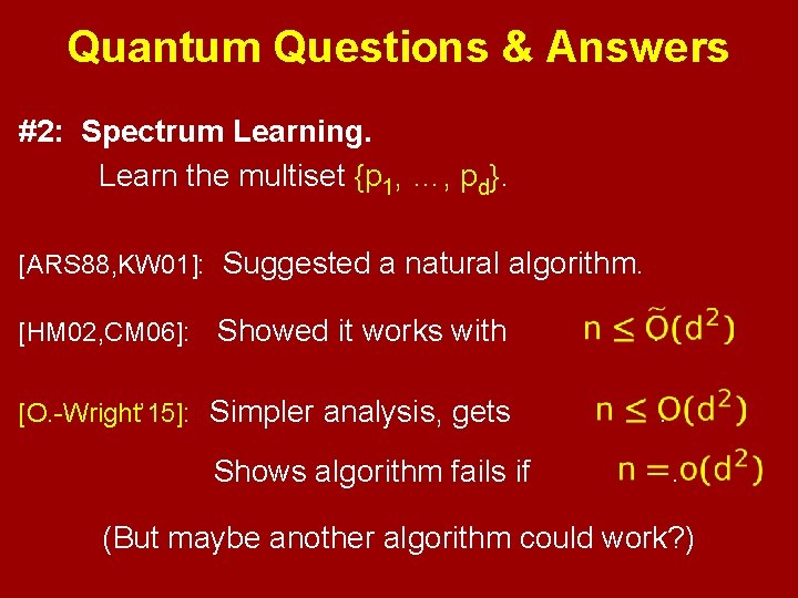
Quantum Questions & Answers #2: Spectrum Learning. Learn the multiset {p 1, …, pd}. [ARS 88, KW 01]: Suggested a natural algorithm. Showed it works with . [O. -Wright’ 15]: Simpler analysis, gets . [HM 02, CM 06]: Shows algorithm fails if . (But maybe another algorithm could work? )

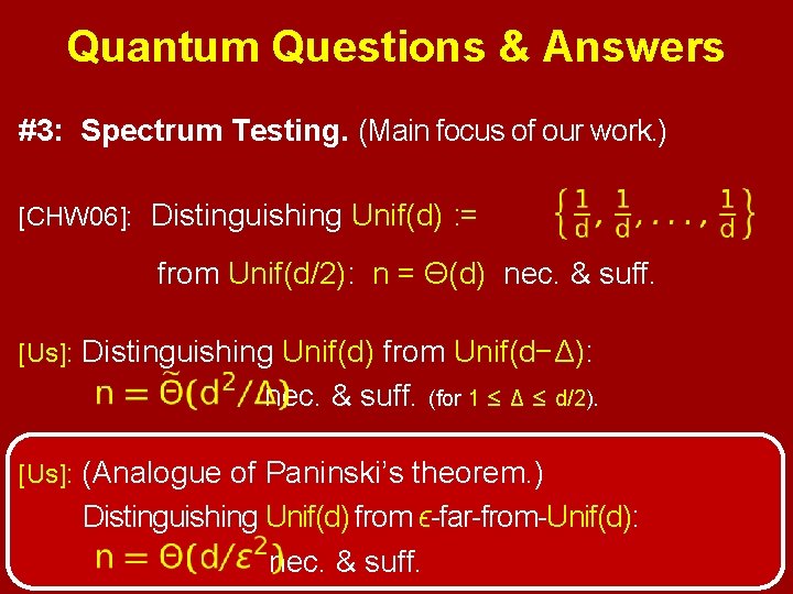
Quantum Questions & Answers #3: Spectrum Testing. (Main focus of our work. ) [CHW 06]: Distinguishing Unif(d) : = from Unif(d/2): n = Θ(d) nec. & suff. [Us]: Distinguishing Unif(d) from Unif(d−Δ): nec. & suff. (for 1 ≤ Δ ≤ d/2). [Us]: (Analogue of Paninski’s theorem. ) Distinguishing Unif(d) from ϵ-far-from-Unif(d): nec. & suff.

Plan for rest of the talk Not going to prove any of theorems. Just going to try to explain the setup. Will start by explaining quantum measurement.

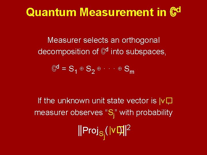
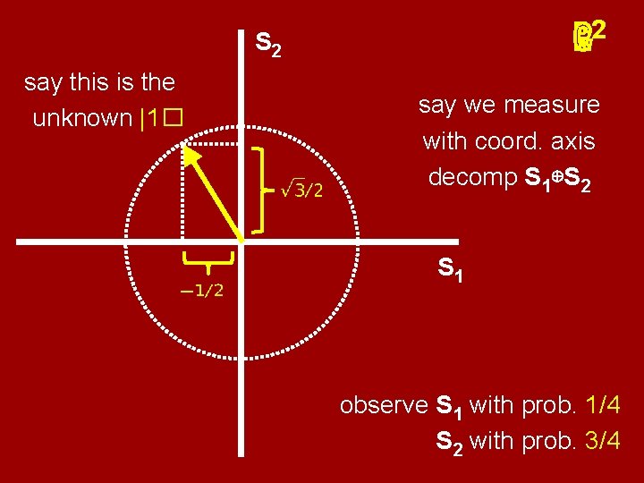
Quantum Measurement in d ℂ Measurer selects an orthogonal decomposition of ℂd into subspaces, ℂd = S 1 ⊕ S 2 ⊕ · · · ⊕ Sm If the unknown unit state vector is |v� , measurer observes “Sj” with probability ||Proj Sj( |v� )||2

2 ℝℂ S 2 say this is the unknown |1� say we measure with coord. axis decomp S 1⊕S 2 S 1 observe S 1 with prob. 1/4 S 2 with prob. 3/4

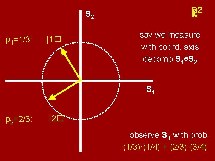
2 ℝ S 2 say this is the |1� p 1 unknown =1/3: say we measure with coord. axis decomp S 1⊕S 2 S 1 p 2=2/3: |2� observe S 1 with prob. (1/3)·(1/4) + (2/3)·(3/4)

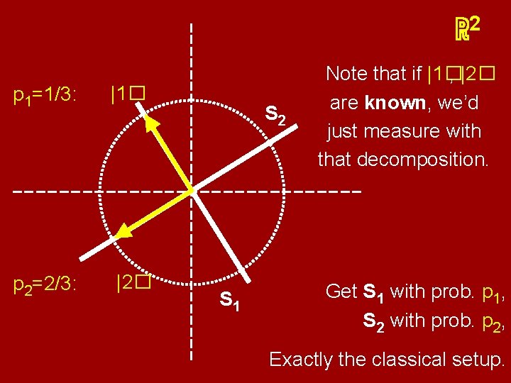
2 ℝ say this is the |1� p 1 unknown =1/3: p 2=2/3: |2� S 2 S 1 Note that if |1� , |2� are known, we’d just measure with that decomposition. Get S 1 with prob. p 1, S 2 with prob. p 2, Exactly the classical setup.

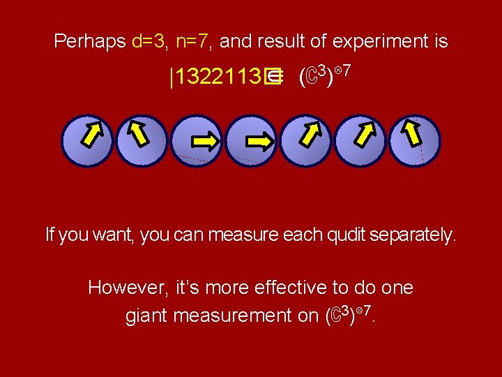
Perhaps d=3, n=7, and result of experiment is |1� |3� |2� |1� |3�∈ (ℂ3)⊗ 7

Perhaps d=3, n=7, and result of experiment is |1� |3� |2� |1322113� |1� |3�∈ (ℂ3)⊗ 7

Perhaps d=3, n=7, and result of experiment is |1� |3� |2� |1322113� |1� |3�∈ (ℂ3)⊗ 7 If you want, you can measure each qudit separately. However, it’s more effective to do one giant measurement on (ℂ3)⊗ 7.

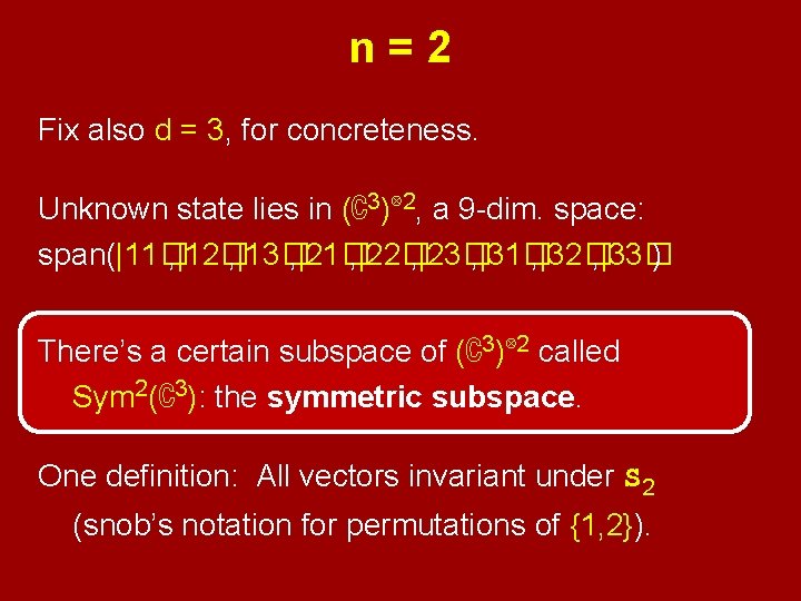
n=2 Fix also d = 3, for concreteness. Unknown state lies in (ℂ3)⊗ 2, a 9 -dim. space: span(|11� , |12� , |13� , |21� , |22� , |23� , |31� , |32� , |33� ) There’s a certain subspace of (ℂ3)⊗ 2 called Sym 2(ℂ3): the symmetric subspace. One definition: All vectors invariant under S 2 (snob’s notation for permutations of {1, 2}).

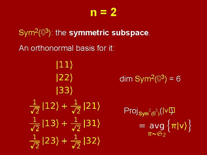
n=2 Sym 2(ℂ3): the symmetric subspace. An orthonormal basis for it: dim Sym 2(ℂ3) = 6 Proj Sym 2(ℂ3)( |v� )

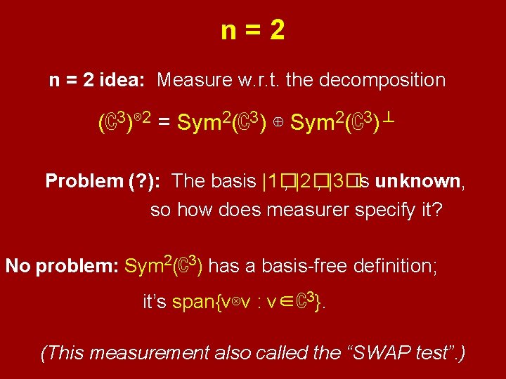
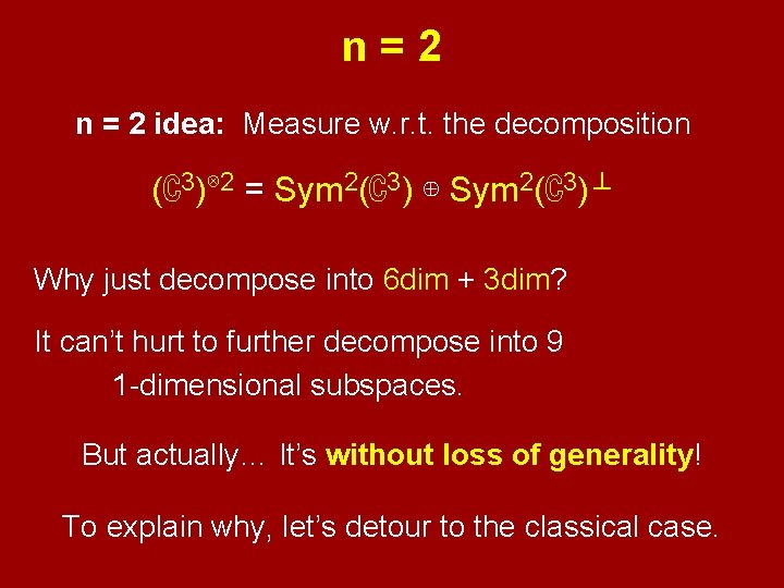
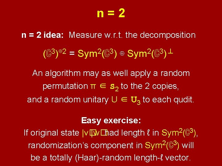
n=2 n = 2 idea: Measure w. r. t. the decomposition (ℂ3)⊗ 2 = Sym 2(ℂ3) ⊕ Sym 2(ℂ3)⊥ Problem (? ): The basis |1� , |2� , |3�is unknown, so how does measurer specify it? No problem: Sym 2(ℂ3) has a basis-free definition; it’s span{v⊗v : v∈ℂ3}. (This measurement also called the “SWAP test”. )

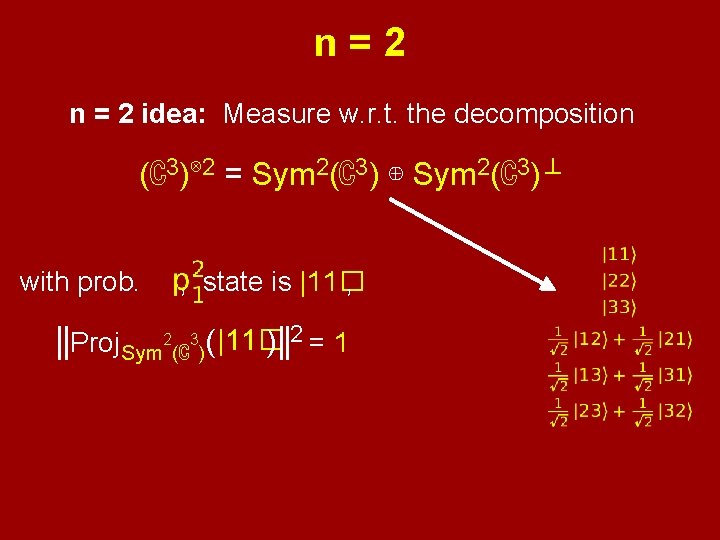
n=2 n = 2 idea: Measure w. r. t. the decomposition (ℂ3)⊗ 2 = Sym 2(ℂ3) ⊕ Sym 2(ℂ3)⊥ with prob. , state is |11� , ||Proj Sym 2(ℂ3)( |11� )||2 = 1

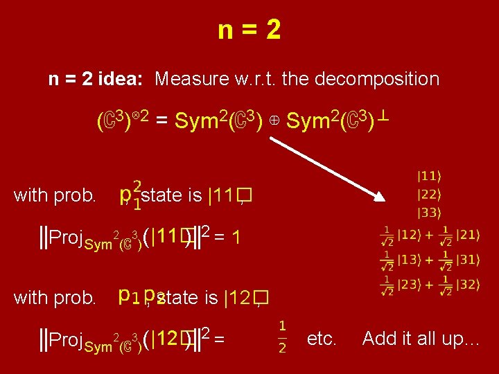
n=2 n = 2 idea: Measure w. r. t. the decomposition (ℂ3)⊗ 2 = Sym 2(ℂ3) ⊕ Sym 2(ℂ3)⊥ with prob. , state is |11� , ||Proj Sym 2(ℂ3)( |11� )||2 = 1 with prob. , state is |12� , ||Proj Sym 2(ℂ3)( |12� )||2 = etc. Add it all up…

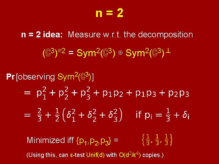
n=2 n = 2 idea: Measure w. r. t. the decomposition (ℂ3)⊗ 2 = Sym 2(ℂ3) ⊕ Sym 2(ℂ3)⊥ Pr [observing Sym 2(ℂ3)] Minimized iff {p 1, p 2, p 3} = {1, 3, 1}. (Using this, can ϵ-test Unif(d) with O(d 2/ϵ 4) copies. )

n=2 n = 2 idea: Measure w. r. t. the decomposition (ℂ3)⊗ 2 = Sym 2(ℂ3) ⊕ Sym 2(ℂ3)⊥ Why just decompose into 6 dim + 3 dim? It can’t hurt to further decompose into 9 1 -dimensional subspaces. But actually… It’s without loss of generality! To explain why, let’s detour to the classical case.

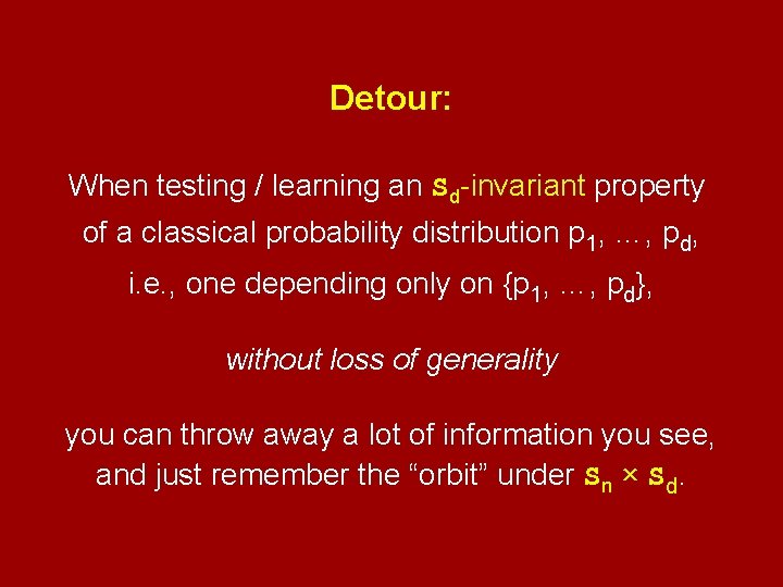
Detour: When testing / learning an Sd-invariant property of a classical probability distribution p 1, …, pd, i. e. , one depending only on {p 1, …, pd}, without loss of generality you can throw away a lot of information you see, and just remember the “orbit” under Sn × Sd.

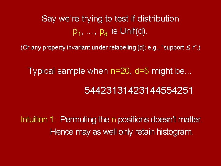
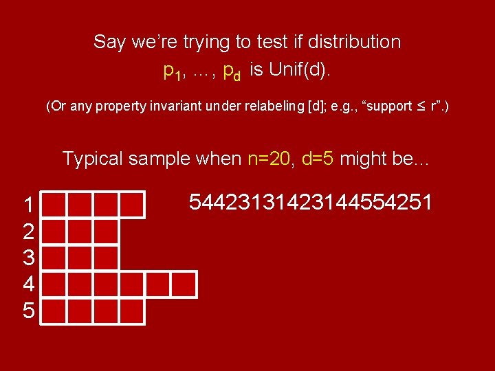
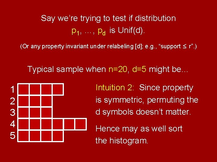
Say we’re trying to test if distribution p 1, …, pd is Unif(d). (Or any property invariant under relabeling [d]; e. g. , “support ≤ r”. ) Typical sample when n=20, d=5 might be… 54423131423144554251 Intuition 1: Permuting the n positions doesn’t matter. Hence may as well only retain histogram.

Say we’re trying to test if distribution p 1, …, pd is Unif(d). (Or any property invariant under relabeling [d]; e. g. , “support ≤ r”. ) Typical sample when n=20, d=5 might be… 1 2 3 4 5 54423131423144554251

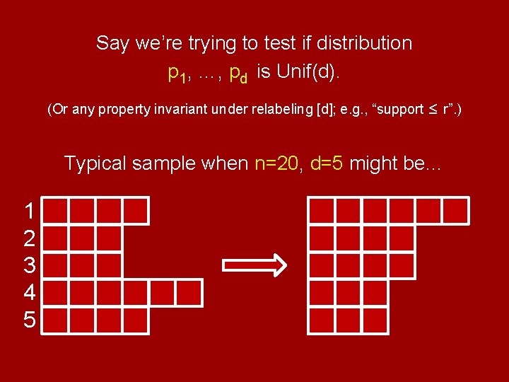
Say we’re trying to test if distribution p 1, …, pd is Unif(d). (Or any property invariant under relabeling [d]; e. g. , “support ≤ r”. ) Typical sample when n=20, d=5 might be… 1 2 3 4 5 Intuition 2: Since property is symmetric, permuting the d symbols doesn’t matter. Hence may as well sort the histogram.

Say we’re trying to test if distribution p 1, …, pd is Unif(d). (Or any property invariant under relabeling [d]; e. g. , “support ≤ r”. ) Typical sample when n=20, d=5 might be… 1 2 3 4 5

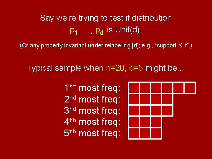
Say we’re trying to test if distribution p 1, …, pd is Unif(d). (Or any property invariant under relabeling [d]; e. g. , “support ≤ r”. ) Typical sample when n=20, d=5 might be… 1 st most freq: 2 nd most freq: 3 rd most freq: 4 th most freq: 5 th most freq:

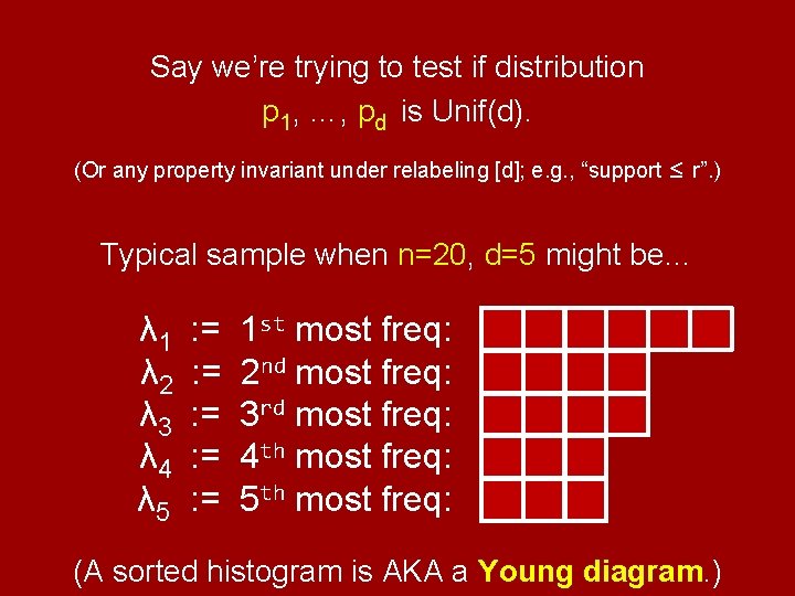
Say we’re trying to test if distribution p 1, …, pd is Unif(d). (Or any property invariant under relabeling [d]; e. g. , “support ≤ r”. ) Typical sample when n=20, d=5 might be… λ 1 λ 2 λ 3 λ 4 λ 5 : = : = : = 1 st most freq: 2 nd most freq: 3 rd most freq: 4 th most freq: 5 th most freq: (A sorted histogram is AKA a Young diagram. )

Claim: An n-sample algorithm for testing an “Sd-invariant” property of p 1, …, pd (one depending only on {p 1, …, pd}) may ignore full sample and just retain the sorted histogram (Young diagram). Formal proof: If algorithm succeeds with high probability, can check it also succeeds with equally high probability if it first blindly applies a random perm from Sn to the positions and a random perm from Sd to the symbols. But then conditioned on the sorted histogram of the sample it sees, the sample is uniformly random among those with that sorted histogram. So an algorithm that only sees the sorted histogram can also succeed with equally high probability.

By the way, for a given sorted histogram / Young diagram λ = (λ 1, λ 2, …, λd), Pr [observing λ] is a nice symmetric polynomial in p 1, …, pd depending on λ.

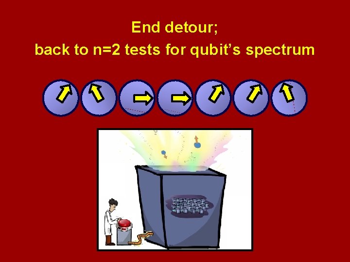
End detour; back to n=2 tests for qubit’s spectrum

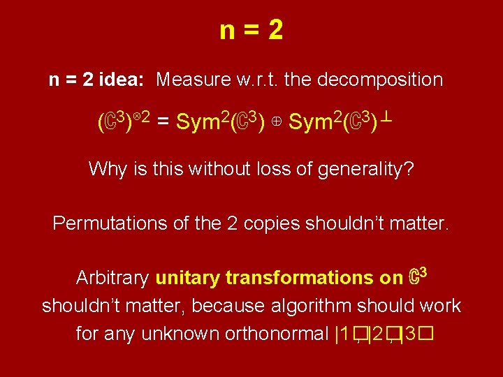
n=2 n = 2 idea: Measure w. r. t. the decomposition (ℂ3)⊗ 2 = Sym 2(ℂ3) ⊕ Sym 2(ℂ3)⊥ Why is this without loss of generality? Permutations of the 2 copies shouldn’t matter. Arbitrary unitary transformations on ℂ3 shouldn’t matter, because algorithm should work for any unknown orthonormal |1� , |2� , |3�.

n=2 n = 2 idea: Measure w. r. t. the decomposition (ℂ3)⊗ 2 = Sym 2(ℂ3) ⊕ Sym 2(ℂ3)⊥ An algorithm may as well apply a random permutation π ∈ S 2 to the 2 copies, and a random unitary U ∈ U 3 to each qudit. Easy exercise: If original state |v� |w�had length ℓ in Sym 2(ℂ3), randomization’s component in Sym 2(ℂ3) will be a totally (Haar)-random length-ℓ vector.

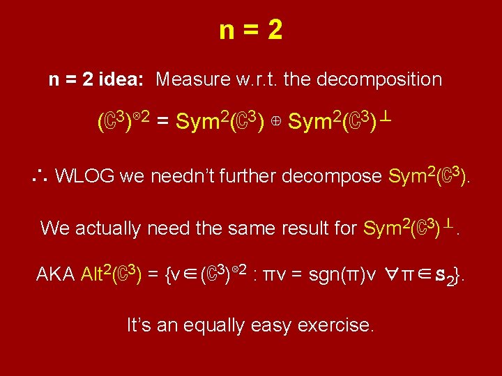
n=2 n = 2 idea: Measure w. r. t. the decomposition (ℂ3)⊗ 2 = Sym 2(ℂ3) ⊕ Sym 2(ℂ3)⊥ ∴ WLOG we needn’t further decompose Sym 2(ℂ3). We actually need the same result for Sym 2(ℂ3)⊥. AKA Alt 2(ℂ3) = {v∈(ℂ3)⊗ 2 : πv = sgn(π)v ∀π∈S 2}. It’s an equally easy exercise.

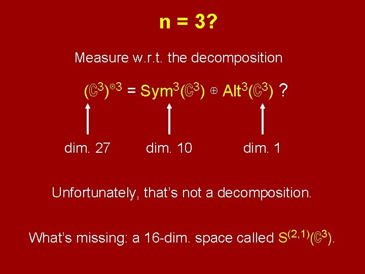
? n = 3? Measure w. r. t. the decomposition ? (ℂ3)⊗ 3 = Sym 3(ℂ3) ⊕ Alt 3(ℂ3) ? dim. 27 dim. 10 dim. 1 Unfortunately, that’s not a decomposition. What’s missing: a 16 -dim. space called S(2, 1)(ℂ3).

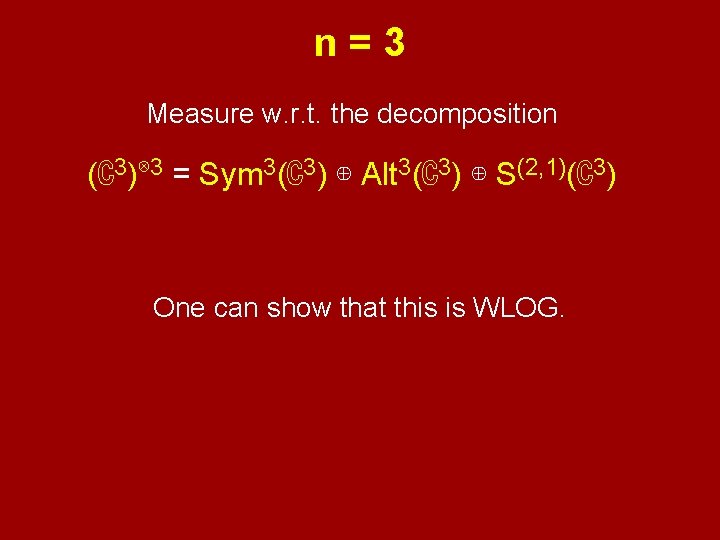
n=3 Measure w. r. t. the decomposition (ℂ3)⊗ 3 = Sym 3(ℂ3) ⊕ Alt 3(ℂ3) ⊕ S(2, 1)(ℂ3) One can show that this is WLOG.

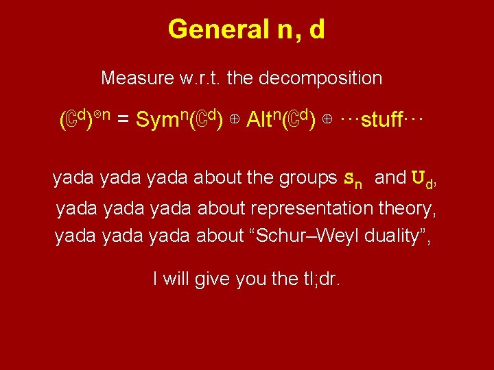
General n, d Measure w. r. t. the decomposition (ℂd)⊗n = Symn(ℂd) ⊕ Altn(ℂd) ⊕ ···stuff··· yada about the groups Sn and Ud, yada about representation theory, yada about “Schur–Weyl duality”, I will give you the tl; dr.

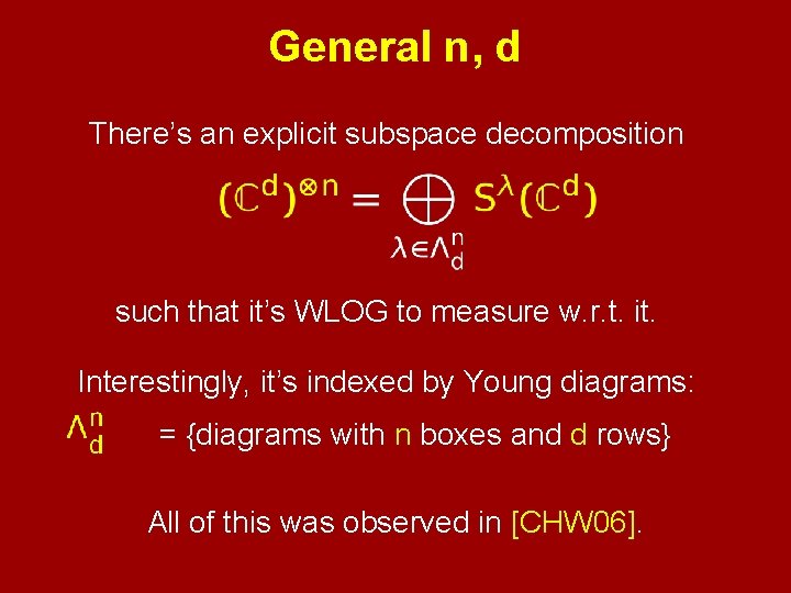
General n, d There’s an explicit subspace decomposition such that it’s WLOG to measure w. r. t. it. Interestingly, it’s indexed by Young diagrams: = {diagrams with n boxes and d rows} All of this was observed in [CHW 06].

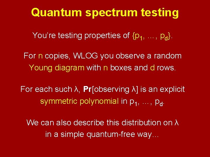
Quantum spectrum testing You’re testing properties of {p 1, …, pd}. For n copies, WLOG you observe a random Young diagram with n boxes and d rows. For each such λ, Pr[observing λ] is an explicit symmetric polynomial in p 1, …, pd. We can also describe this distribution on λ in a simple quantum-free way…

The distribution on λ Pick w ~ [d]n with symbols probs. i. i. d. p 1, …, pd. n=20, d = 5 e. g. : w = 54423131423144554251 Classical testing: you just get to see w.

The distribution on λ Pick w ~ [d]n with symbols probs. i. i. d. p 1, …, pd. n=20, d = 5 e. g. : w = 54423131423144554251 Quantum testing: you see λ defined by… λ 1 = longest incr. subseq λ 1 + λ 2 = longest union of 2 incr. subseqs λ 1 + λ 2 + λ 3 = longest union of 3 incr. subseqs ··· λ 1 + λ 2 + λ 3 + · · · + λd = n

The distribution on λ Pick w ~ [d]n with symbols probs. i. i. d. p 1, …, pd. n=20, d = 5 e. g. : w = 54423131423144554251 Quantum testing: you see λ defined by… 54423131423144554251 54423131423144554251 (Alternatively, you see “RSK”(w). )

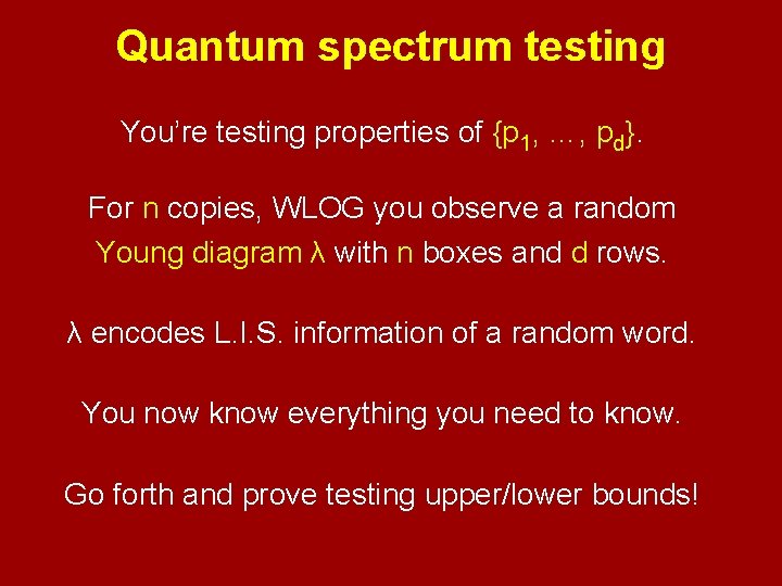
Quantum spectrum testing You’re testing properties of {p 1, …, pd}. For n copies, WLOG you observe a random Young diagram λ with n boxes and d rows. λ encodes L. I. S. information of a random word. You now know everything you need to know. Go forth and prove testing upper/lower bounds!

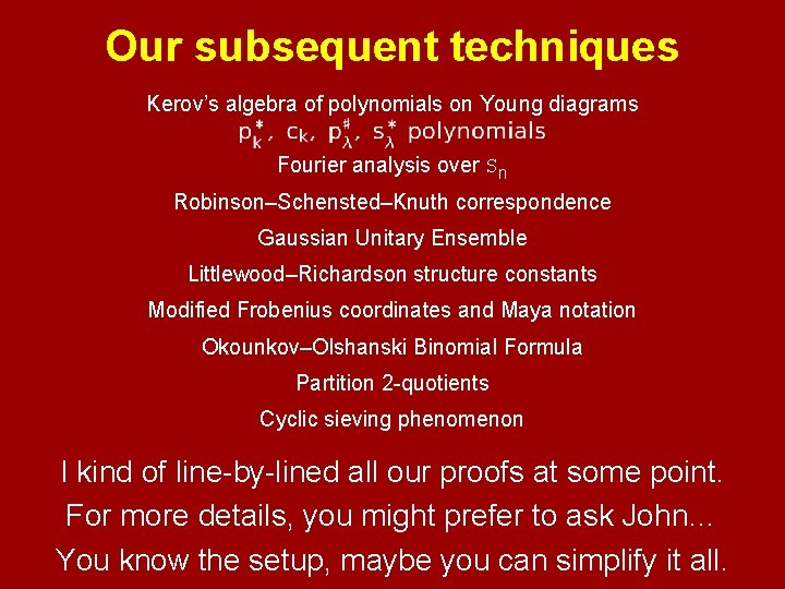
Our subsequent techniques Kerov’s algebra of polynomials on Young diagrams Fourier analysis over Sn Robinson–Schensted–Knuth correspondence Gaussian Unitary Ensemble Littlewood–Richardson structure constants Modified Frobenius coordinates and Maya notation Okounkov–Olshanski Binomial Formula Partition 2 -quotients Cyclic sieving phenomenon I kind of line-by-lined all our proofs at some point. For more details, you might prefer to ask John… You know the setup, maybe you can simplify it all.

Thanks!