Computational Applications of Noise Sensitivity Ryan ODonnell Includes

Computational Applications of Noise Sensitivity Ryan O’Donnell

Includes joint work with: Elchanan Mossel Rocco Servedio Adam Klivans Nader Bshouty Oded Regev Benny Sudakov

Intro to Noise Sensitivity

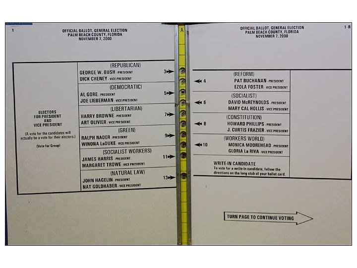
Election schemes • suppose there is an election between two parties, called 0 and 1 • assume unrealistically that n voters cast votes independently and unif. randomly • an election scheme is a boolean function f : {0, 1}n → {0, 1} mapping votes to winner • what if there are errors in recording of votes? suppose each vote is misrecorded independently with prob. ε.

Election schemes • suppose there is an election between two parties, called 0 and 1 • assume unrealistically that n voters cast votes independently and unif. randomly • an election scheme is a boolean function f : {0, 1}n → {0, 1} mapping votes to winner • what if there are errors in recording of votes? suppose each vote is misrecorded independently with prob. ε. • what is the prob. this affects elec. ’s outcome?

Definition Let f : {0, 1}n → {0, 1} be any boolean function. Let 0 ≤ ε ≤ ½, the noise rate. Let x be a uniformly randomly chosen string in {0, 1}n, and let y be an ε-noisy version of x. Then the noise sensitivity of f at ε is: NSε(f) = Pr [f(x) ≠ f(y)]. x, y

Examples Suppose f is the constant function f(x) = 1. Then NSε(f) = 0. Suppose f is the “dictator” function f(x) = x 1. Then NSε(f) = ε. In general, for fixed f, NSε(f) is a function of ε.

Examples – parity The parity (xor) function on n bits 1 iff there an odd number of 1’s in the input. In calculating Pr[f(x) ≠ f(y)], it doesn’t matter what x is, just how many flips there are. NSε(PARITYn) = Pr[odd number of heads in n ε-biased coin flips] = ½ – ½(1 – 2ε)n.

NSε(PARITY 10) = ½ – ½(1 – 2ε)10

Basic facts about NS • NSε(f) is an increasing, (log-)concave function of ε which is 0 at 0 and 2 p(1 -p) at ½ (where p=Pr[f = 1]). • this follows from a formula for NSε(f) in terms of Fourier coefficients: NSε(f) = 2 f(Ø) – 2 Σ (1 -2ε)|S| f (S)2. S µ [n]

PARITY, MAJORITY, dictator, and AND on 5 bits

PARITY, MAJORITY, dictator, and AND on 15 bits

PARITY, MAJORITY, dictator, and AND on 45 bits

History of Noise Sensitivity (in computer science)

History of Noise Sensitivity Kahn-Kalai-Linial ’ 88 The Influence of Variables on Boolean Functions

Kahn-Kalai-Linial ’ 88 • implicitly studied noise sensitivity • motivation: study of random walks on the hypercube where the initial distribution is uniform over a subset • the question, “What is the prob. that a random walk of length εn, starting uniformly in f-1(1), ends up outside f-1(1)? ” is essentially asking about NSε(f) • famous for using Fourier analysis and “Bonami-Beckner inequality” in TCS

History of Noise Sensitivity Håstad ’ 97 Some Optimal Inapproximability Results

Håstad ’ 97 • breakthrough hardness of approximation results • decoding the Long Code: given access to the truth-table of a function, want to test that it is “significantly” determined by a “junta” (very small number of variables) • roughly, does a noise sensitivity test: picks x and y as in n. s. , tests f(x)=f(y)

History of Noise Sensitivity Benjamini-Kalai-Schramm ’ 98 Noise Sensitivity of Boolean Functions and Applications to Percolation

Benjamini-Kalai-Schramm ’ 98 • intensive study of noise sensitivity of boolean functions • introduced asymptotic notions of noise sensitivity/stability, related them to Fourier coefficients • studied noise sensitivity of percolation functions, threshold functions • made conjectures connecting noise sensitivity to circuit complexity • and more…

This thesis New noise sensitivity results and applications: • tight noise sensitivity estimates for boolean halfspaces, monotone functions • hardness amplification thms. (for NP) • learning algorithms for halfspaces, DNF (from random walks), juntas • new coin-flipping problem, and use of “reverse” Bonami-Beckner inequality

Hardness Amplification

Hardness on average def: We say f : {0, 1}n → {0, 1} is (1 -ε)-hard for circuits of size s if there is no circuit of size s which computes f correctly on more than (1 -ε)2 n inputs. def: A complexity class is (1 -ε)-hard for polynomial circuits if there is a function family (fn) in the class such that for suff. large n, fn is (1 -ε)-hard for circuits of size poly(n).

Hardness of EXP, NP Of course we can’t show NP is even (1 -2 -n)hard for poly ckts, since this is NPµP/poly. But let’s assume EXP, NP µ P/poly. Then just how hard are these for poly circuits? For EXP, extremely strong results known – [BFNW 93, Imp 95, IW 97, Kv. M 99, STV 99]: if EXP is (1 -2 -n)-hard for poly circuits, then it is (½ + 1/poly(n))-hard for poly circuits. What about NP?

Yao’s XOR Lemma Some of the hardness amplification results for EXP use Yao’s XOR Lemma: Thm: If f is (1 -ε)-hard for poly circuits, then PARITYk f is (½+½(1 -2ε)k)-hard for poly circuits. Here, if f is a boolean fcn on n inputs and g is a boolean fcn on k inputs, g f is the function on kn inputs given by g(f(x 1), …, f(xk)). No coincidence that the hardness bound for PARITYk f is 1 -NSε(PARITYk).

A general direct product thm. Yao doesn’t help for NP – if you have a hard function fn in NP, PARITYk fn probably isn’t in NP. We generalize Yao and determine the hardness of g fn for any g – in terms of the noise sensitivity of g: Thm: If f (balanced) is (1 -ε)-hard for poly circuits, then g fn is roughly (1 -NSε(g))hard for poly circuits.

Why noise sensitivity? Suppose f is balanced and (1 -ε)-hard for poly circuits. x 1, …, xk are chosen uniformly at random, and you, a poly circuit, have to guess g(f(x 1), …, f(xk)). Natural strategy is to try to compute each yi = f(xi) and then guess g(y 1, …, yk). But f is (1 -ε)-hard for you! So Pr[f(xi)≠yi] = ε. Success prob. : Pr[g(f(x 1)…f(xk))=g(y 1…yk)] = 1 -NSε(g).

Hardness of NP If (fn) is a (hard) function family in NP, and (gk) is a monotone function family, then (gk fn) is in NP. We give constructions and prove tight bounds for the problem of finding monotone g such that NSε(g) is very large (close to ½) for ε very small. Thm: If NP is (1 -1/poly(n))-hard for poly ckts, then NP is (½ + 1/√n)-hard for poly ckts.

Learning algorithms

Learning theory ([Valiant 84]) deals with the following scenario: • someone holds an n-bit boolean function f • you know f belongs to some class of fcns (eg, {parities of subsets}, {poly size DNF}) • you are given a bunch of uniformly random labeled examples, (x, f(x)) • you must efficiently come up with a hypothesis function h that predicts f well

Learning noise-stable functions We introduce a new idea for showing function classes are learnable: Noise-stable classes are efficiently learnable Thm: Suppose C is a class of boolean fcns on n bits, and for all f ∈ C, NSε(f) ≤ β(ε). Then there is an alg. for learning C to within accuracy ε in time: -1 n. O(1)/β (ε).

Example – halfspaces E. g. , using [Peres 98], every boolean function f which is the “intersection of two halfspaces” has NSε(f) ≤ O(√ε). Cor: The class of “intersections of two halfspaces” can be learned in time n. O(1/ε²). No previously known subexponential alg. We also analyze the noise sensitivity of some more complicated classes based on halfspaces and get learning algs. for them.

Why noise stability? Suppose a function is fairly noise stable. In some sense this means if you know f(x), you have a good guess for f(y) for y’s which are somewhat close to x in Hamming distance. Idea: Draw a “net” of examples: (x 1, f(x 1)), … (x. M, f(x. M)). To hypothesize about y, compute a weighted average of known labels, based on dist. to y: hypothesis =… sgn[ w(Δ(y, x 1))f(x 1) + ··· + w(Δ(y, x. M))f(x. M) ].

Learning from random walks Holy grail of learning: Learn poly size DNF formulas in polynomial time. Consider natural weakening of learning: examples not iid, come from random walk. We show DNF poly-time learnable in this model. Indeed, also in a harder model: “NS-model”: examples are (x, f(x), y, f(y)) Proof: estimate NS on subsets of input bits ⇒ find large Fourier coefficients.

Learning juntas The essential blocking issue for learning poly size DNF formulas is that they can be O(log n)-juntas. Previously, no known algorithm for learning k-juntas in time better than the trivial nk. We give the first improvement: algorithm runs in time n. 704 k. Can the strong relationship between juntas and noise sensitivity improve this?

Coin flipping

The T 1 -2ε operator T 1 -2ε operates on the space of functions {0, 1}n → R: T 1 -2ε(f) (x) = E [f(y)] (= Pr[f(y) = 1]). y = noiseε(x) Notable fact about T 1 -2ε: the Bonami-Beckner [Bon 68] “hypercontractive” inequality: ||Tλ(f)||2 ≤ ||f||1+λ²

Bonami, Beckner

The T 1 -2ε operator It follows easily that: NSε(f) = ½ - ½ ||T√ 1 -2ε(f)||2. Thus studying noise sensitivity is equivalent to studying the (2 -)norm of the T 1 -2ε operator. We consider studying higher norms of the T 1 -2ε operator. The problem can be phrased combinatorially, in terms of a natural coin flipping problem.

“Cosmic coin flipping” • n random votes cast in an election • we use a balanced election scheme, f • k different auditors get copies of the votes; however, each gets an ε-noisy copy • what is the probability all k auditors agree on the winner of the election? Equivalently, k distributed parties want to flip a shared random coin given noisy access to a “cosmic” random string.

Relevance of the problem Application of this scenario: “Everlasting security” of [Ding. Rabin 01] – a cryptographic protocol assuming that many distributed parties have access to a satellite broadcasting stream of random bits. Also a natural error-correction problem: without encoding, can parties attain some shared entropy?

Success as function of k Most interesting asymptotic case: ε a small constant, n unbounded, k → ∞. What is the maximum success probability? Surprisingly, goes to 0 only polynomially: Thm: The best success probability of k players is Õ(1/k 4ε), with the majority function being essentially optimal.

Reverse Bonami-Beckner To prove that no protocol can do better than k-Ω(1), we need to use a reverse Bonami. Beckner inequality [Bor 82]: for f ≥ 0, t ≥ 0, ||Tλ(f)||1 -t/λ ≥ ||f||1 -tλ Concentration of measure interpretation: Let A be a reasonably large subset of the cube. Then almost all x have Pr[y ∈ A] somewhat large.

Conclusions

Open directions • estimate the noise sensitivity of various classes of functions – general intersections of threshold functions, percolation functions, … • new hardness of approx. results using NSjunta connection [DS 02, Kho 02, DF 03? ]… • find a substantially better algorithm for learning juntas • explore applications of reverse Bonami. Beckner – coding theory, e. g. ?