Analysis of Boolean Functions Ryan ODonnell Carnegie Mellon

Analysis of Boolean Functions Ryan O’Donnell Carnegie Mellon University

Part 1: A. Fourier expansion basics B. Concepts: Bias, Influences, Noise Sensitivity C. Kalai’s proof of Arrow’s Theorem

10 Minute Break

Part 2: A. The Hypercontractive Inequality B. Algorithmic Gaps

Sadly no time for: Learning theory Pseudorandomness Arithmetic combinatorics Random graphs / percolation Communication complexity Metric / Banach spaces Coding theory etc.

1 A. Fourier expansion basics

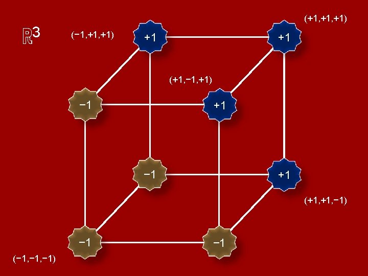
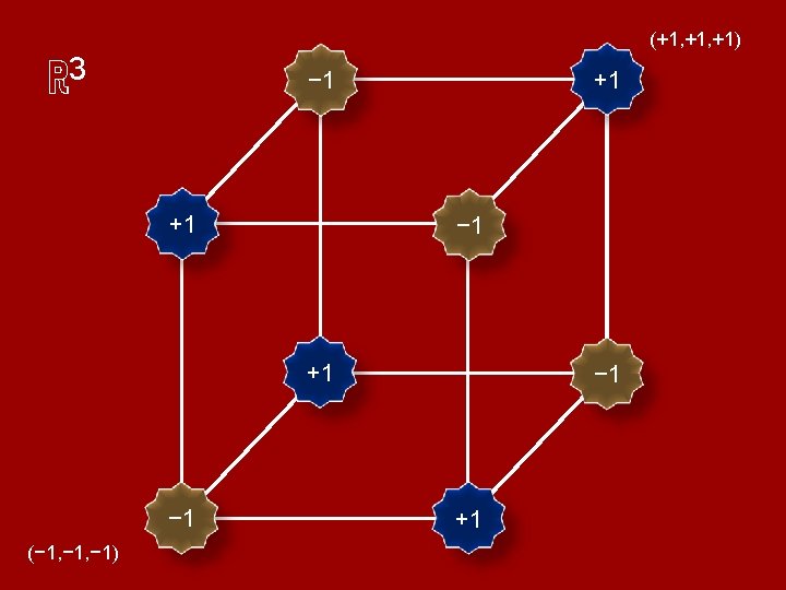
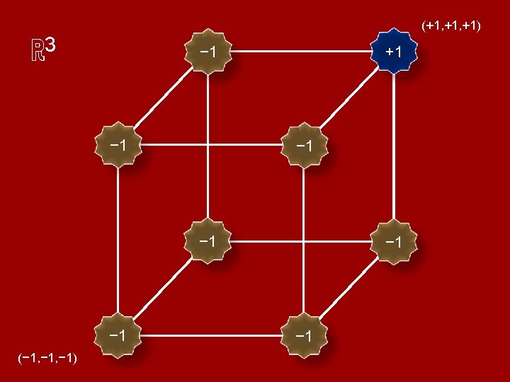
f : {0, 1}n {0, 1}


 Every f : {− 1, +1}n {− 1, +1} can")
Proposition: (indeed, → ℝ) Every f : {− 1, +1}n {− 1, +1} can be expressed as a multilinear polynomial, That’s it. That’s the “Fourier expansion” of f. (u niq ue ly )
 Every f : {− 1, +1}n {− 1, +1} can")
Proposition: (indeed, → ℝ) Every f : {− 1, +1}n {− 1, +1} can be expressed as a multilinear polynomial, That’s it. That’s the “Fourier expansion” of f. (u niq ue ly )

⇓ Rest: 0

Why? Coefficients encode useful information. When? 1. Uniform probability involved 2. Hamming distances relevant

Parseval’s Theorem: Let f : {− 1, +1}n {− 1, +1}. Then avg { f(x)2 }
![“Weight” of f on S ⊆ [n] =](http://slidetodoc.com/presentation_image_h2/7a8f21adeb7a3b2e7b6c854c690d1c50/image-28.jpg "“Weight” of f on S ⊆ [n] =")
“Weight” of f on S ⊆ [n] =


1 B. Concepts: Bias, Influences, Noise Sensitivity

Social Choice: Candidates ± 1 n voters Votes are random f : {− 1, +1}n {− 1, +1} is the “voting rule”
![Bias of f: avg f(x) = Pr[+1 wins] − Pr[− 1 wins] Fact: Weight](http://slidetodoc.com/presentation_image_h2/7a8f21adeb7a3b2e7b6c854c690d1c50/image-37.jpg "Bias of f: avg f(x) = Pr[+1 wins] − Pr[− 1 wins] Fact: Weight")
Bias of f: avg f(x) = Pr[+1 wins] − Pr[− 1 wins] Fact: Weight on ∅ = measures “imbalance”.
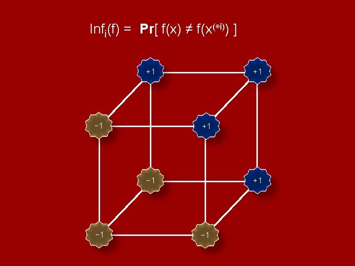
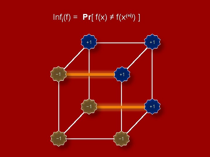
![Influence of i on f: Pr[ f(x) ≠ f(x(⊕i)) ] = Pr[voter i is](http://slidetodoc.com/presentation_image_h2/7a8f21adeb7a3b2e7b6c854c690d1c50/image-38.jpg "Influence of i on f: Pr[ f(x) ≠ f(x(⊕i)) ] = Pr[voter i is")
Influence of i on f: Pr[ f(x) ≠ f(x(⊕i)) ] = Pr[voter i is a swing voter] Fact:
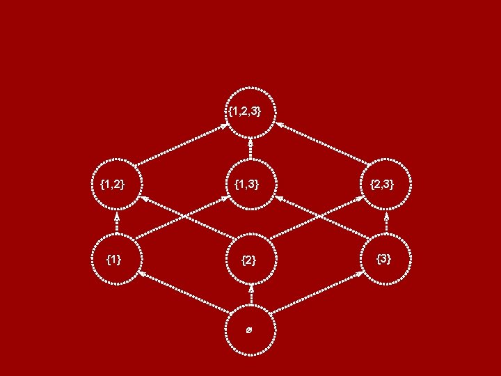
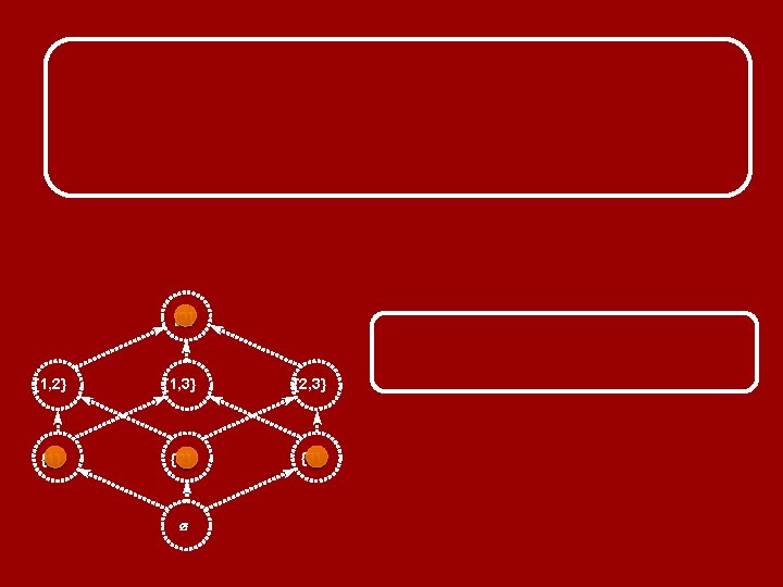
 {1, 2, 3} {1, 2} {1, 3} {2,")
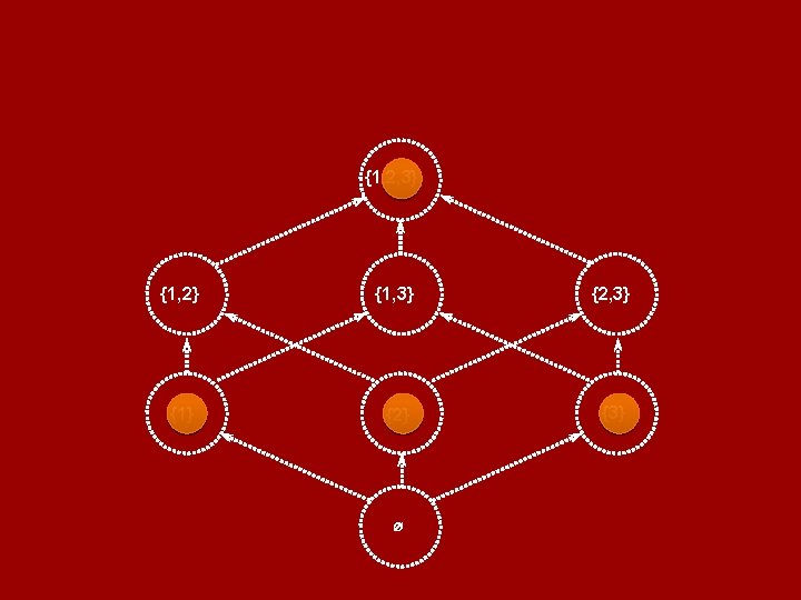
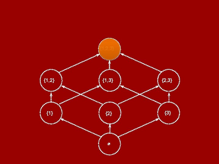
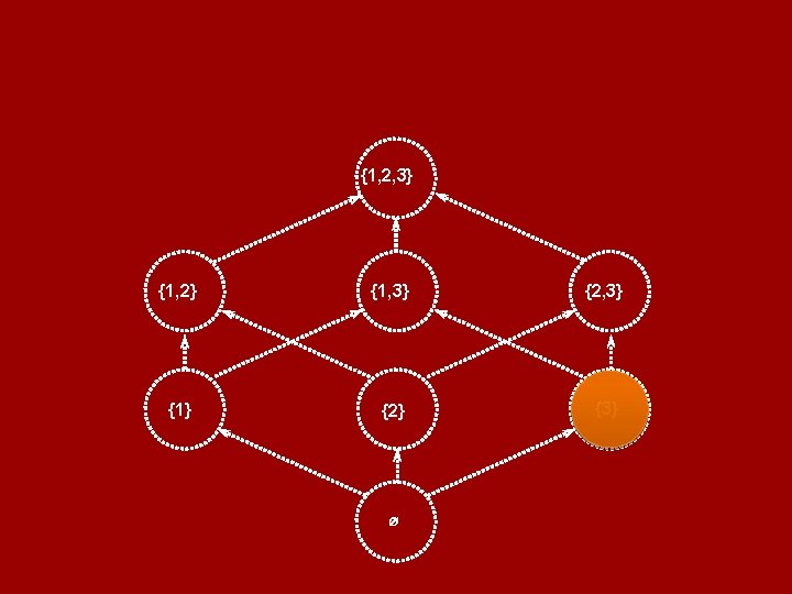
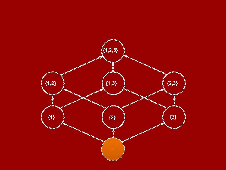
Maj(x 1, x 2, x 3) {1, 2, 3} {1, 2} {1, 3} {2, 3} {1} {2} {3} ∅

 = frac. of edges which are cut edges")
avg Infi(f) = frac. of edges which are cut edges
")
LMN Theorem: If then f is in AC 0 avg Infi(f)
 ⇒ Parity ∉ AC 0 ⇒ avg Infi(Majn) = ⇒ Majority")
⇒ avg Infi(Parityn) ⇒ Parity ∉ AC 0 ⇒ avg Infi(Majn) = ⇒ Majority ∉ AC 0 = 1
 = 0, then Corollary: Assuming f monotone, − 1 or")
KKL Theorem: If Bias(f) = 0, then Corollary: Assuming f monotone, − 1 or +1 can bribe o(n) voters and win w. p. 1−o(1).
![Noise Sensitivity of f at ϵ: NSԑ(f) = Pr[wrong winner wins], when each vote](http://slidetodoc.com/presentation_image_h2/7a8f21adeb7a3b2e7b6c854c690d1c50/image-47.jpg "Noise Sensitivity of f at ϵ: NSԑ(f) = Pr[wrong winner wins], when each vote")
Noise Sensitivity of f at ϵ: NSԑ(f) = Pr[wrong winner wins], when each vote misrecorded w/prob ϵ f( + − + + − − ) f( − − + + + − − )

![Learning Theory principle: [LMN’ 93, …, KKMS’ 05] If all f ∈ C have](http://slidetodoc.com/presentation_image_h2/7a8f21adeb7a3b2e7b6c854c690d1c50/image-49.jpg "Learning Theory principle: [LMN’ 93, …, KKMS’ 05] If all f ∈ C have")
Learning Theory principle: [LMN’ 93, …, KKMS’ 05] If all f ∈ C have small NSԑ(f) then C is efficiently learnable.

Proposition: 1 for small ԑ, with Electoral College: 0 ϵ 1

1 C. Kalai’s proof of Arrow’s Theorem
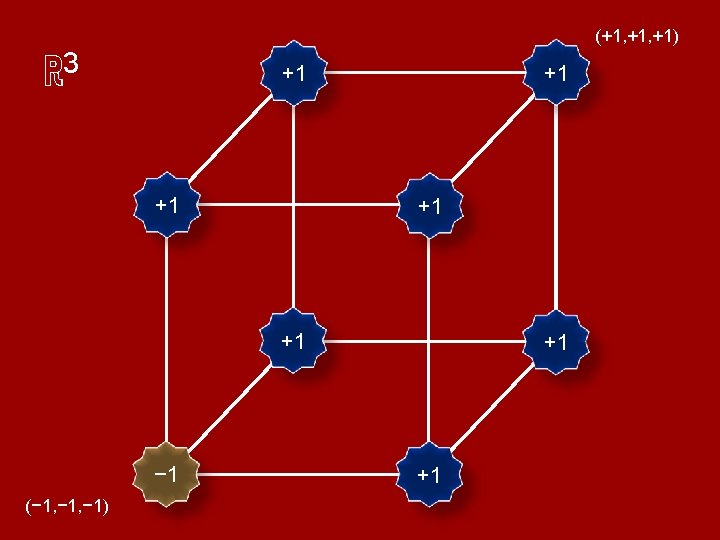
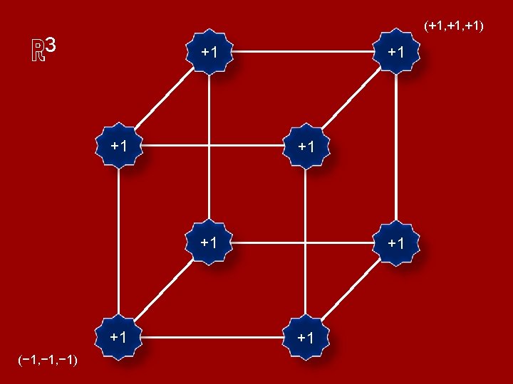
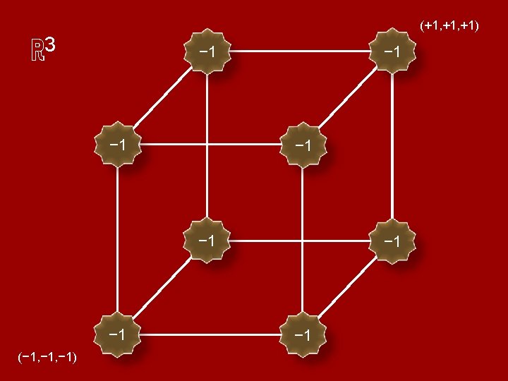
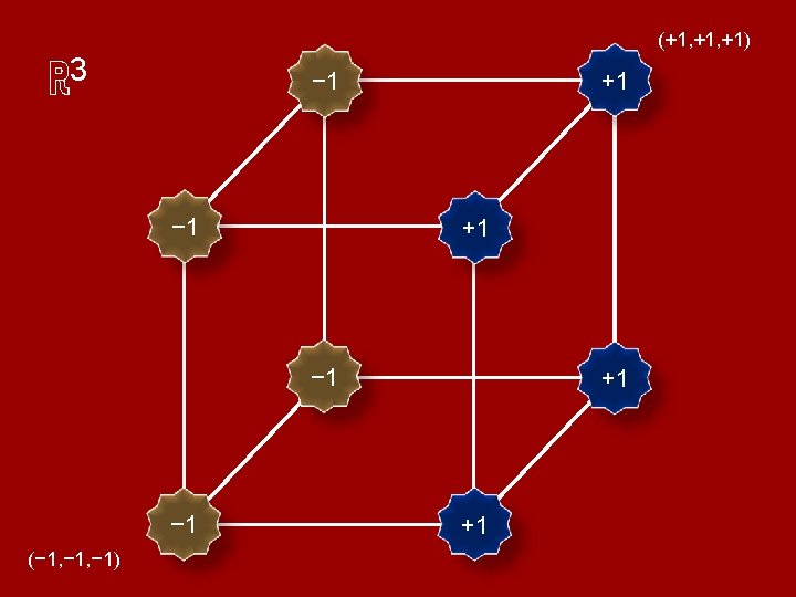
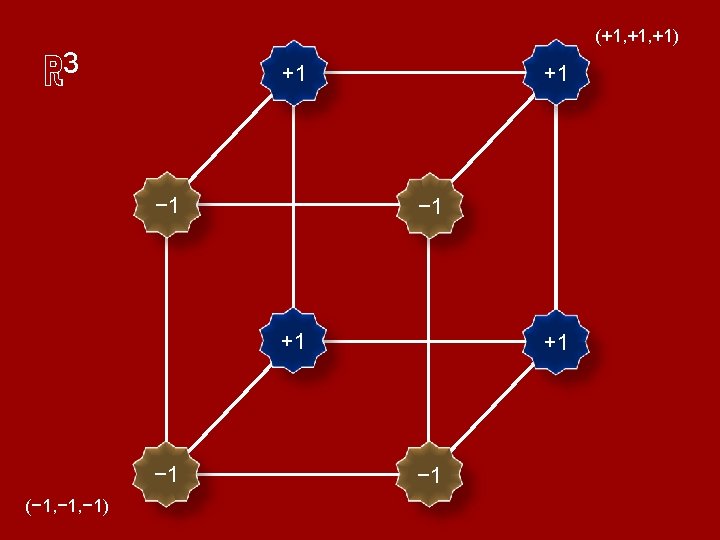
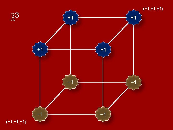
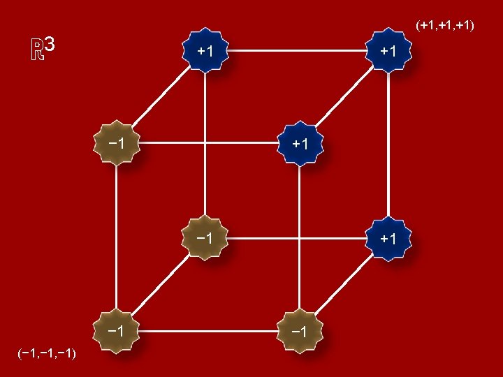
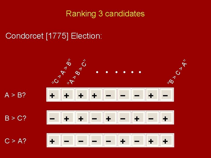
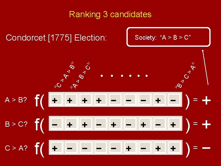
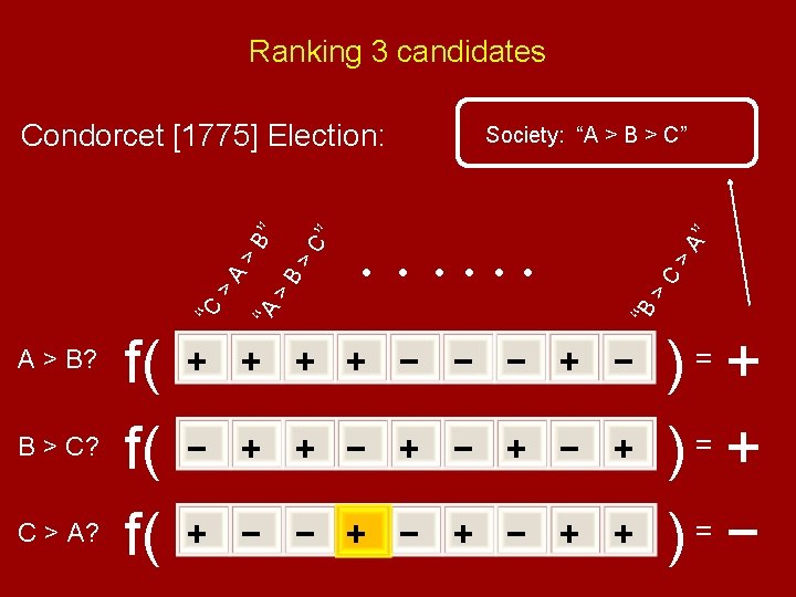
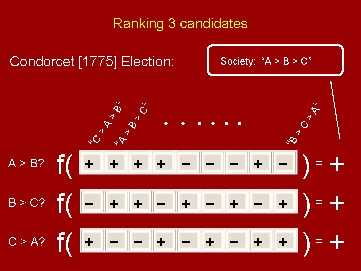
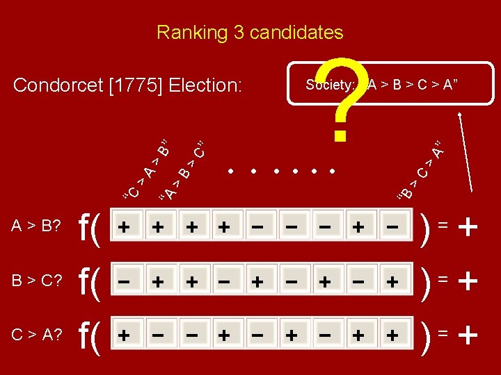
![Ranking 3 candidates Condorcet [1775] Election: A > B? B > C? C >](http://slidetodoc.com/presentation_image_h2/7a8f21adeb7a3b2e7b6c854c690d1c50/image-53.jpg "Ranking 3 candidates Condorcet [1775] Election: A > B? B > C? C >")
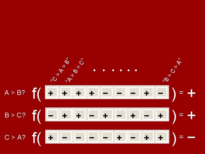
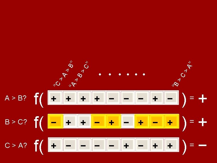
Ranking 3 candidates Condorcet [1775] Election: A > B? B > C? C > A?
![Arrow’s Impossibility Theorem [1950]: If f : {− 1, +1}n {− 1, +1} never](http://slidetodoc.com/presentation_image_h2/7a8f21adeb7a3b2e7b6c854c690d1c50/image-59.jpg "Arrow’s Impossibility Theorem [1950]: If f : {− 1, +1}n {− 1, +1} never")
Arrow’s Impossibility Theorem [1950]: If f : {− 1, +1}n {− 1, +1} never gives irrational outcome in Condorcet elections, then f is a Dictator or a negated-Dictator.
![Gil Kalai’s Proof [2002]:](http://slidetodoc.com/presentation_image_h2/7a8f21adeb7a3b2e7b6c854c690d1c50/image-60.jpg "Gil Kalai’s Proof [2002]:")
Gil Kalai’s Proof [2002]:

Gil Kalai’s Proof:

Gil Kalai’s Proof:

Gil Kalai’s Proof, concluded: f never gives irrational outcomes ⇒ equality ⇒ all Fourier weight “at level 1” ⇒ f(x) = ±xj for some j (exercise).
![⇓ Guilbaud’s Number ≈. 912 Guilbaud’s Theorem [1952]](http://slidetodoc.com/presentation_image_h2/7a8f21adeb7a3b2e7b6c854c690d1c50/image-66.jpg "⇓ Guilbaud’s Number ≈. 912 Guilbaud’s Theorem [1952]")
⇓ Guilbaud’s Number ≈. 912 Guilbaud’s Theorem [1952]
![Corollary of “Majority Is Stablest” [MOO 05]: Infi(f) ≤ o(1) for all i, If](http://slidetodoc.com/presentation_image_h2/7a8f21adeb7a3b2e7b6c854c690d1c50/image-67.jpg "Corollary of “Majority Is Stablest” [MOO 05]: Infi(f) ≤ o(1) for all i, If")
Corollary of “Majority Is Stablest” [MOO 05]: Infi(f) ≤ o(1) for all i, If then Pr[rational outcome with f]

10 minute break

Part 2: A. The Hypercontractive Inequality B. Algorithmic Gaps

2 A. The Hypercontractive Inequality AKA Bonami-Beckner Inequality

KKL Theorem Friedgut’s Theorem Talagrand’s Theorem Every monotone graph property has a sharp threshold FKN Theorem Bourgain’s Junta Theorem Majority Is Stablest Theorem all use “Hypercontractive Inequality”

Hoeffding Inequality: Let F = c 0 + c 1 x 1 + c 2 x 2 + ··· + cn xn, where xi’s are indep. , unif. random ± 1.

Hoeffding Inequality: Let F = c 0 + c 1 x 1 + c 2 x 2 + ··· + cn xn, Mean: μ = c 0 Variance:

Hypercontractive Inequality*: Let Mean: μ = Variance:

Hypercontractive Inequality: Let Then for all q ≥ 2,

Hypercontractive Inequality: Let Then F is a “reasonabled” random variable.

Hypercontractive Inequality: Let Then for all q ≥ 2,

“q = 4” Hypercontractive Inequality: Let Then

“q = 4” Hypercontractive Inequality: Let Then

KKL Theorem Friedgut’s Theorem Talagrand’s Theorem Every monotone graph property has a sharp threshold FKN Theorem Bourgain’s Junta Theorem Majority Is Stablest Theorem all use Hypercontractive Inequality

KKL Theorem Friedgut’s Theorem Talagrand’s Theorem Every monotone graph property has a sharp threshold FKN Theorem Bourgain’s Junta Theorem Majority Is Stablest Theorem just use “q = 4” Hypercontractive Inequality

“q = 4” Hypercontractive Inequality: Let F be degree d over n i. i. d. ± 1 r. v. ’s. Then Proof [MOO’ 05]: Induction on n. Obvious step. Use induction hypothesis. Use Cauchy-Schwarz on the obvious thing. Use induction hypothesis. Obvious step.

2 B. Algorithmic Gaps
” best poly-time guarantee ln(N) Opt")
“Set-Cover is NP-hard to approximate to factor ln(N)” best poly-time guarantee ln(N) Opt
 Algorithmic Gap for LP-Rand-Rounding” LP-Rand-Rounding guarantee ln(N) Opt")
“Factor ln(N) Algorithmic Gap for LP-Rand-Rounding” LP-Rand-Rounding guarantee ln(N) Opt
 ln(N) Opt(S)")
“Algorithmic Gap Instance S for LP-Rand-Rounding” LP-Rand-Rounding(S) ln(N) Opt(S)

Algorithmic Gap instances are often “based on” {− 1, +1}n.

Sparsest-Cut: Algorithm: Arora-Rao-Vazirani SDP. Guarantee: Factor

Opt = 1/n

Opt = 1/n

Opt = 1/n
 = sgn( )")
Opt = 1/n f(x) = sgn( )
 = sgn(r 1 x 1 + • •")
Opt = 1/n ARV gets f(x) = sgn(r 1 x 1 + • • • + rnxn)

Opt = 1/n ARV gets gap:

Algorithmic Gaps → Hardness-of-Approx LP / SDP-rounding Alg. Gap instance • n optimal “Dictator” solutions • “generic mixture of Dictators” much worse + PCP technology = same-gap hardness-of-approximation

Algorithmic Gaps → Hardness-of-Approx LP / SDP-rounding Alg. Gap instance • n optimal “Dictator” solutions • “generic mixture of Dictators” much worse + PCP technology = same-gap hardness-of-approximation
 ≤ 1/n. 01 for all")
KKL / Talagrand Theorem: If f is balanced, Infi(f) ≤ 1/n. 01 for all i, then avg Infi(f) ≥ Gap: Θ(log n) = Θ(log N).
![[CKKRS 05]: KKL + Unique Games Conjecture ⇒ Ω(log log N) hardness-of-approx.](http://slidetodoc.com/presentation_image_h2/7a8f21adeb7a3b2e7b6c854c690d1c50/image-99.jpg "[CKKRS 05]: KKL + Unique Games Conjecture ⇒ Ω(log log N) hardness-of-approx.")
[CKKRS 05]: KKL + Unique Games Conjecture ⇒ Ω(log log N) hardness-of-approx.

2 -Colorable 3 -Uniform hypergraphs: Input: 2 -colorable, 3 -unif. hypergraph Output: 2 -coloring Obj: Max. fraction of legally colored hyperedges
![2 -Colorable 3 -Uniform hypergraphs: Algorithm: SDP [KLP 96]. Guarantee: [Zwick 99]](http://slidetodoc.com/presentation_image_h2/7a8f21adeb7a3b2e7b6c854c690d1c50/image-101.jpg "2 -Colorable 3 -Uniform hypergraphs: Algorithm: SDP [KLP 96]. Guarantee: [Zwick 99]")
2 -Colorable 3 -Uniform hypergraphs: Algorithm: SDP [KLP 96]. Guarantee: [Zwick 99]
")
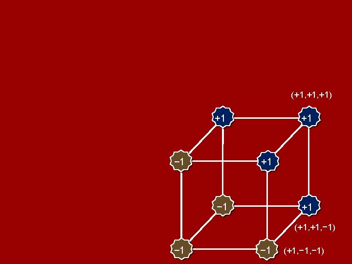
Algorithmic Gap Instance Vertices: {− 1, +1}n 6 n hyperedges: { (x, y, z) : poss. prefs in a Condorcet election} (i. e. , triples s. t. (xi, yi, zi) NAE for all i)
 = f")
Elts: {− 1, +1}n 2 -coloring Edges: Condorcet votes (x, y, z) = f : {− 1, +1}n → {− 1, +1} frac. legally colored hyperedges = Pr[“rational” outcome with f] Instance 2 -colorable? ✔ (2 n optimal solutions: ±Dictators)
 SDP rounding alg. may")
Elts: {− 1, +1}n Edges: Condorcet votes (x, y, z) SDP rounding alg. may output f(x) = sgn(r 1 x 1 + • • • + rnxn) Random weighted majority also rational-with-prob. -. 912! [same CLT arg. ]

Algorithmic Gaps → Hardness-of-Approx LP / SDP-rounding Alg. Gap instance • n optimal “Dictator” solutions • “generic mixture of Dictators” much worse + PCP technology = same-gap hardness-of-approximation
 ≤ o(1) for all i, If then Pr[rational")
Corollary of Majority Is Stablest: Infi(f) ≤ o(1) for all i, If then Pr[rational outcome with f] Cor: this + Unique Games Conjecture ⇒. 912 hardness-of-approx*

2 C. Future Directions

Develop the “structure vs. pseudorandomness” theory for Boolean functions.

Thanks!
- Slides: 109