Invariance Principles in Theoretical Computer Science Ryan ODonnell

Invariance Principles in Theoretical Computer Science Ryan O’Donnell Carnegie Mellon University

Talk Outline 1. Describe some TCS results requiring variants of the Central Limit Theorem. 2. Show a flexible proof of the CLT with error bounds. 3. Open problems and an advertisement.

Talk Outline 1. Describe some TCS results requiring variants of the Central Limit Theorem. 2. Show a flexible proof of the CLT with error bounds. 3. Open problems and an advertisement.

Linear Threshold Functions

Linear Threshold Functions

Learning Theory Servedio’ 08] Thm : [O- Can learn LTFs f in poly(n) time, just from correlations Key: when all |c i | ≤ ϵ. E[f( x)xi ].

Property Testing Servedio’ 09] Thm : [Matulef-O-Rubinfeld- Can test if ϵ-close to an LTF with poly(1/ Key: when all |c i | ≤ ϵ. ϵ) querie

Derandomization Zuckerman’ 10] Thm : [Meka- PRG for LTFs with seed length O(log(n) log(1/ ϵ)). Key: even when xi ’s not fully independent.

Multidimensional CLT? For when all small compared to

Derandomization+ Zuckerman’ 10] Thm : [Gopalan-O-Wu- PRG for “functions of O(1) LTFs” with seed length O(log(n) log(1/ Key: ϵ)). Derandomized multidimensional CLT.

Property Testing+ [Blais -O’ 10] Thm : Testing if Majority of k bits needs k is a Ω(1) queries. Key: assuming E[Xi ] = E[Yi ], Var[ Xi ] = Var[ Yi ], and some other conditions. (actually, a multidimensional version)

Social Choice, Inapproximability Oleszkiewicz’ 05] Thm : [Mossel-O- a) Among voting schemes where no voter has unduly large influence, Majority is most robust to noise. b) Max-Cut is UG-hard to. 878 -approx. Key: If P is a low-deg. multilin. polynomial, assuming P has “small coeffs. on each coord. ”

Talk Outline 1. Describe some TCS results requiring variants of the Central Limit Theorem. 2. Show a flexible proof of the CLT with error bounds. 3. Open problems and an advertisement.

Gaussians Standard Gaussian: G ~ N(0, 1). Mean 0, Var Anti-concentration: Pr[ G ∈ [u− ϵ, u+ ϵ] ] ≤ O a + b G also a “Gaussian”: N(a, b 2) Sum of independent Gaussians is Gaussian: If G ~ N(a, b 2 ), H ~ N(c, d 2 ) are independen then G + H ~ N(a+c, b 2 +d 2 ).

Central Limit Theorem (CLT) X 1 , X 2 , X 3 , … independent, ident. distrib. , mean 0, variance σ 2,

CLT with error bounds X 1 , X 2 , …, Xn independent, ident. distrib. , mean 0, variance 1/n, X 1 + · · · + Xn is “close to” N(0, 1), assuming Xi is not too wacky:

Niceness of random variables Say E[X] = 0, stddev[ X] = σ. def : ( ≥ σ). “ def ”: X is “ nice ” if eg : not nice : ± 1. N(0, 1). Unif on [-a, a].

Niceness of random variables Say E[X] = 0, stddev[ X] = σ. def : ( def : eg : not nice : ≥ σ). X is “ C-nice ” if ± 1. N(0, 1). Unif on [-a, a].

Berry-Esseen Theorem X 1 , X 2 , …, Xn independent, ident. distrib. , mean 0, variance 1/n, X 1 + · · · + Xn is ϵ-close to N(0, 1), assuming Xi is C-nice , where [Shevtsova’ 07]: Y “ ϵ-close” to Z: . 7056

General Case X 1 , X 2 , …, Xn independent, ident. distrib. , mean 0, X 1 + · · · + Xn is ϵ-close to N(0, 1), assuming Xi is C-nice ,

Berry-Esseen: How to prove? X 1 , X 2 , …, Xn indep. , mean 0, S = X 1 + · · · + Xn ϵ-close to G ~ N(0, 1). 1. “Characteristic functions” 2. “Stein’s method” 3. “Replacement” = think like a cryptographer

Indistinguishability of random variables S “ ϵ-close” to G:

Indistinguishability of random variables S “ ϵ-close” to G: u

Indistinguishability of random variables S “ ϵ-close” to G: t u

Indistinguishability of random variables S “ ϵ-close” to G:

Replacement method S “ ϵ-close” to G: u δ

Replacement method X 1 , X 2 , …, Xn indep. , mean 0, S = X 1 + · · · + Xn G ~ N(0, 1) For smooth

Replacement method Hybrid argument X 1 , X 2 , …, Xn indep. , mean 0, S = X 1 + · · · + Xn G = G 1 + · · · + Gn For smooth

Invariance principle X 1 , X 2 , …, Xn Y 1 , Y 2 , …, Yn indep. , mean 0, Var[ Xi ] = Var[ Yi ] = SX = X 1 + · · · + X n S Y = Y 1 + · · · + Yn For smooth

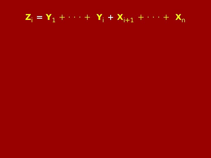
Hybrid argument X 1 , X 2 , …, Xn , Y 1 , Y 2 , …, Yn , independent matching means and variances. SX = X 1 + · · · + Xn vs. SY = Y 1 + · · · + Yn Def : Zi = Y 1 + · · · + Yi + Xi+1 + · · · + Xn S X = Z 0 , S Y = Zn

Hybrid argument X 1 , X 2 , …, Xn , Y 1 , Y 2 , …, Yn , independent matching means and variances. Zi = Y 1 + · · · + Yi + Xi+1 + · · · + Xn Goal:

Zi = Y 1 + · · · + Yi + Xi+1 + · · · + Xn where U = Y 1 + · · · + Yi− 1 + Xi+1 + · · · + Xn Note: U, Xi , Yi independent. Goal:

− = ∴ by indep. and matching means/variances!

Variant Berry-Esseen: Say If X 1 , X 2 , …, Xn & Y 1 , Y 2 , …, Yn indep. and have matching means/variances, then

Usual Berry-Esseen: If X 1 , X 2 , …, Xn indep. , mean 0, Hack u δ

Usual Berry-Esseen: If X 1 , X 2 , …, Xn indep. , mean 0, Variant Berry-Esseen + Hack Usual Berry-Esseen except with error O( ϵ 1/4 )

Extensions are easy! Vector-valued version: Use multidimensional Taylor theorem. Derandomized version: If X 1 , …, Xm C-nice, 3 -wise indep. , then X 1 +···+ Xm is O(C)-nice. Higher-degree version: X 1 , …, Xm C-nice, indep. , Q is a deg. -d poly. , then Q( X 1 , …, Xm ) is O(C) d -nice.

Talk Outline 1. Describe some TCS results requiring variants of the Central Limit Theorem. 2. Show a flexible proof of the CLT with error bounds. 3. Open problems, advertisement, anecdote?

Open problems 1. Recover usual Berry-Esseen via the Replacement method. 2. Vector-valued: Get correct dependence on test sets K. ( Gaussian surface area 3. Higher-degree: improve (? ) the exponential dependence 4. Find more applications on degree d. in TCS. ? )

Do you like LTFs and PTFs ? Do you like probability and geometry ? Oct. 21 -22 (“ just before FOCS ”) workshop at the Princeton Intractability Center: Analysis and Geometry of Boolean Threshold Functions Diakonikolas! Kane! Meka! Rubinfeld! Servedio! Shpilka! Vempala! And more! http: //intractability. princeton. edu/blog/2010/08/workshop-ltfptf/