Process Control Designing Process and Control Systems for

Process Control: Designing Process and Control Systems for Dynamic Performance Chapter 3. Mathematical Modelling Principles Copyright © Thomas Marlin 2013 The copyright holder provides a royalty-free license for use of this material at non-profit educational institutions

CHAPTER 3 : MATHEMATICAL MODELLING PRINCIPLES When I complete this chapter, I want to be able to do the following. • Formulate dynamic models based on fundamental balances • Solve simple first-order linear dynamic models • Determine how key aspects of dynamics depend on process design and operation

CHAPTER 3 : MATHEMATICAL MODELLING PRINCIPLES Outline of the lesson. • Reasons why we need dynamic models • Six (6) - step modelling procedure • Many examples - mixing tank - CSTR - draining tank • General conclusions about models • Workshop

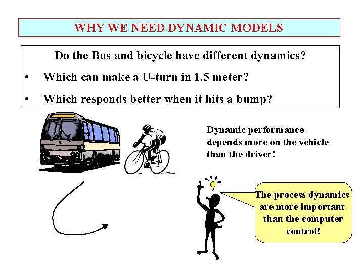
WHY WE NEED DYNAMIC MODELS Do the Bus and bicycle have different dynamics? • Which can make a U-turn in 1. 5 meter? • Which responds better when it hits a bump? Dynamic performance depends more on the vehicle than the driver! The process dynamics are more important than the computer control!

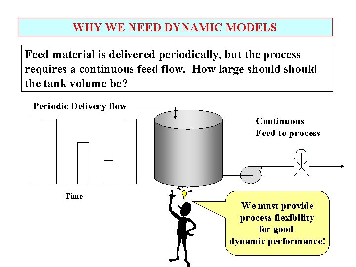
WHY WE NEED DYNAMIC MODELS Feed material is delivered periodically, but the process requires a continuous feed flow. How large should the tank volume be? Periodic Delivery flow Continuous Feed to process Time We must provide process flexibility for good dynamic performance!

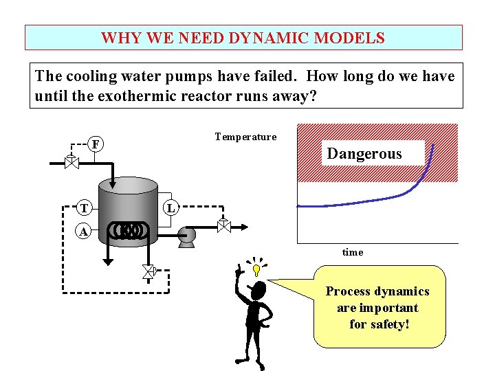
WHY WE NEED DYNAMIC MODELS The cooling water pumps have failed. How long do we have until the exothermic reactor runs away? Temperature F T Dangerous L A time Process dynamics are important for safety!

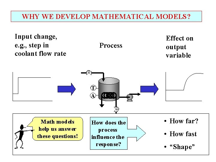
WHY WE DEVELOP MATHEMATICAL MODELS? Input change, e. g. , step in coolant flow rate Process Effect on output variable T A Math models help us answer these questions! How does the process influence the response? • How far? • How fast • “Shape”

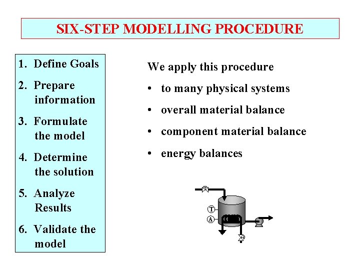
SIX-STEP MODELLING PROCEDURE 1. Define Goals We apply this procedure 2. Prepare information • to many physical systems 3. Formulate the model • component material balance 4. Determine the solution 5. Analyze Results 6. Validate the model • overall material balance • energy balances T A

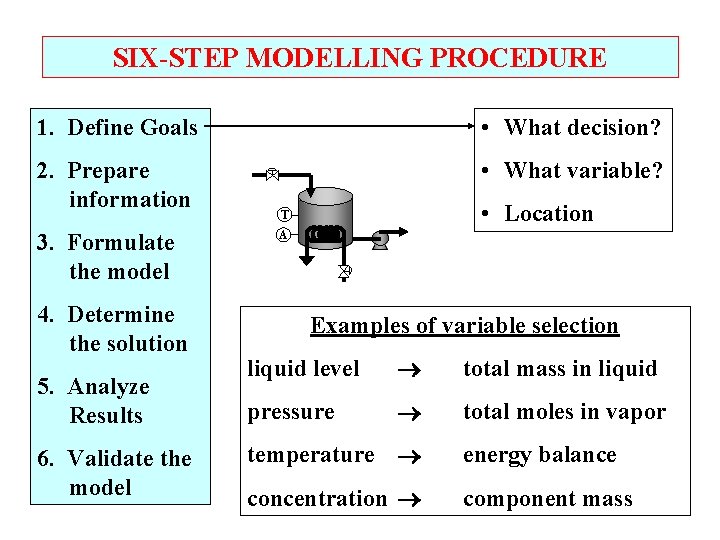
SIX-STEP MODELLING PROCEDURE 1. Define Goals • What decision? 2. Prepare information • What variable? 3. Formulate the model 4. Determine the solution 5. Analyze Results 6. Validate the model • Location T A Examples of variable selection liquid level total mass in liquid pressure total moles in vapor temperature energy balance concentration component mass

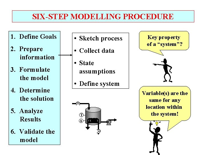
SIX-STEP MODELLING PROCEDURE 1. Define Goals • Sketch process 2. Prepare information • Collect data 3. Formulate the model 4. Determine the solution 5. Analyze Results 6. Validate the model Key property of a “system”? • State assumptions • Define system T A Variable(s) are the same for any location within the system!

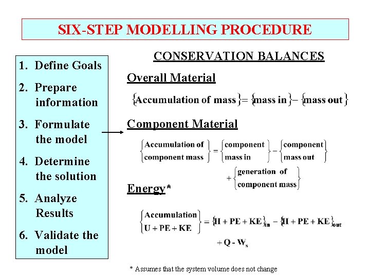
SIX-STEP MODELLING PROCEDURE 1. Define Goals 2. Prepare information 3. Formulate the model 4. Determine the solution 5. Analyze Results CONSERVATION BALANCES Overall Material Component Material Energy* 6. Validate the model * Assumes that the system volume does not change

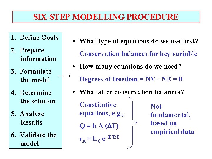
SIX-STEP MODELLING PROCEDURE 1. Define Goals • What type of equations do we use first? 2. Prepare information Conservation balances for key variable 3. Formulate the model 4. Determine the solution 5. Analyze Results 6. Validate the model • How many equations do we need? Degrees of freedom = NV - NE = 0 • What after conservation balances? Constitutive equations, e. g. , Q = h A ( T) r. A = k 0 e -E/RT Not fundamental, based on empirical data

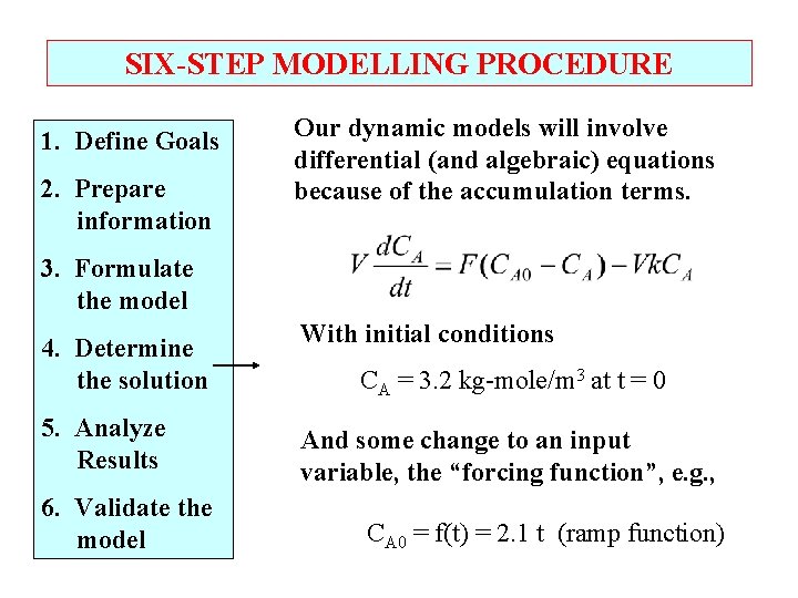
SIX-STEP MODELLING PROCEDURE 1. Define Goals 2. Prepare information Our dynamic models will involve differential (and algebraic) equations because of the accumulation terms. 3. Formulate the model 4. Determine the solution 5. Analyze Results 6. Validate the model With initial conditions CA = 3. 2 kg-mole/m 3 at t = 0 And some change to an input variable, the “forcing function”, e. g. , CA 0 = f(t) = 2. 1 t (ramp function)

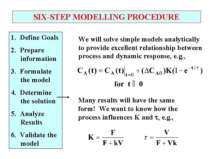
SIX-STEP MODELLING PROCEDURE 1. Define Goals 2. Prepare information We will solve simple models analytically to provide excellent relationship between process and dynamic response, e. g. , 3. Formulate the model 4. Determine the solution 5. Analyze Results 6. Validate the model Many results will have the same form! We want to know how the process influences K and , e. g. ,

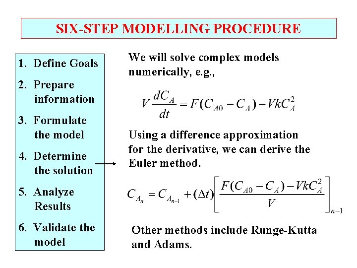
SIX-STEP MODELLING PROCEDURE 1. Define Goals 2. Prepare information 3. Formulate the model 4. Determine the solution We will solve complex models numerically, e. g. , Using a difference approximation for the derivative, we can derive the Euler method. 5. Analyze Results 6. Validate the model Other methods include Runge-Kutta and Adams.

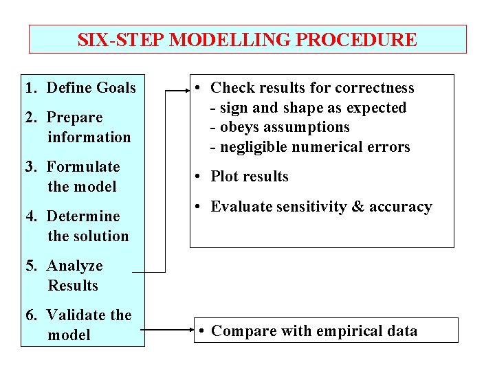
SIX-STEP MODELLING PROCEDURE 1. Define Goals 2. Prepare information 3. Formulate the model 4. Determine the solution • Check results for correctness - sign and shape as expected - obeys assumptions - negligible numerical errors • Plot results • Evaluate sensitivity & accuracy 5. Analyze Results 6. Validate the model • Compare with empirical data

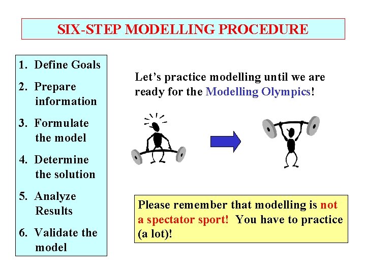
SIX-STEP MODELLING PROCEDURE 1. Define Goals 2. Prepare information Let’s practice modelling until we are ready for the Modelling Olympics! 3. Formulate the model 4. Determine the solution 5. Analyze Results 6. Validate the model Please remember that modelling is not a spectator sport! You have to practice (a lot)!

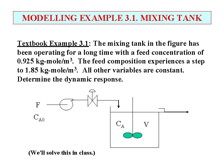
MODELLING EXAMPLE 3. 1. MIXING TANK Textbook Example 3. 1: The mixing tank in the figure has been operating for a long time with a feed concentration of 0. 925 kg-mole/m 3. The feed composition experiences a step to 1. 85 kg-mole/m 3. All other variables are constant. Determine the dynamic response. F CA 0 (We’ll solve this in class. ) CA V

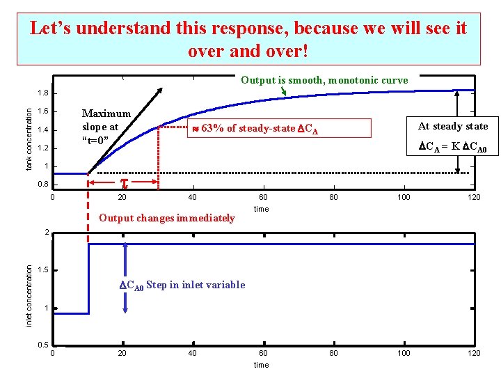
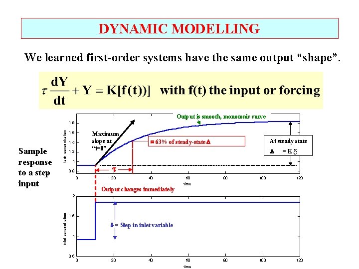
Let’s understand this response, because we will see it over and over! Output is smooth, monotonic curve tank concentration 1. 8 1. 6 Maximum slope at “t=0” 1. 4 1. 2 1 At steady state 63% of steady-state CA = K CA 0 0. 8 0 20 40 Output changes immediately 60 80 100 120 time inlet concentration 2 1. 5 CA 0 Step in inlet variable 1 0. 5 0 20 40 60 time

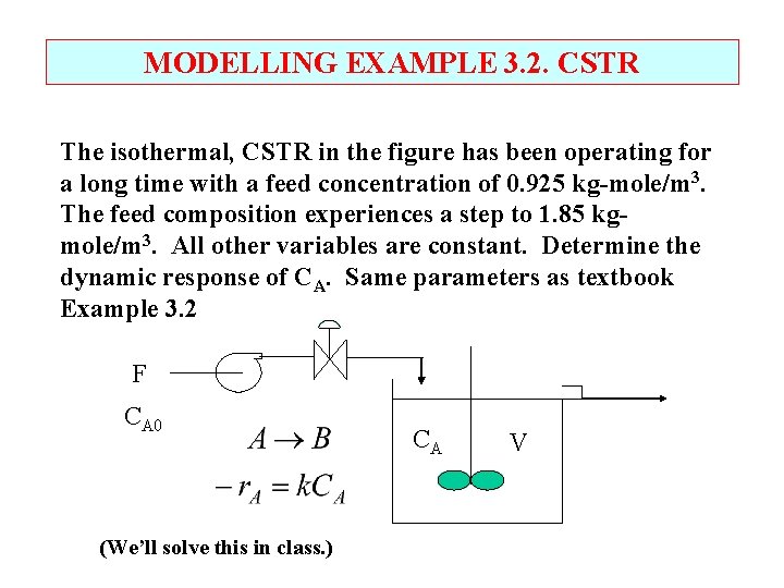
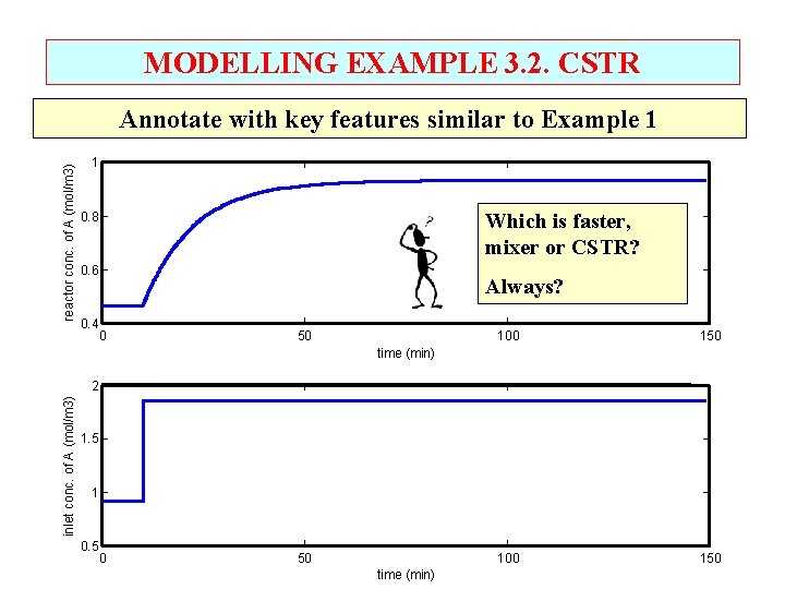
MODELLING EXAMPLE 3. 2. CSTR The isothermal, CSTR in the figure has been operating for a long time with a feed concentration of 0. 925 kg-mole/m 3. The feed composition experiences a step to 1. 85 kgmole/m 3. All other variables are constant. Determine the dynamic response of CA. Same parameters as textbook Example 3. 2 F CA 0 (We’ll solve this in class. ) CA V

MODELLING EXAMPLE 3. 2. CSTR reactor conc. of A (mol/m 3) Annotate with key features similar to Example 1 1 Which is faster, mixer or CSTR? 0. 8 0. 6 0. 4 Always? 0 50 100 150 time (min) inlet conc. of A (mol/m 3) 2 1. 5 1 0. 5 0 50 time (min)

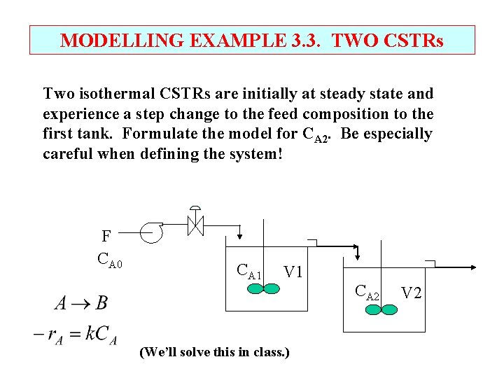
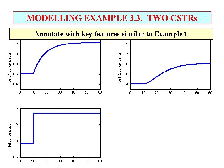
MODELLING EXAMPLE 3. 3. TWO CSTRs Two isothermal CSTRs are initially at steady state and experience a step change to the feed composition to the first tank. Formulate the model for CA 2. Be especially careful when defining the system! F CA 0 CA 1 V 1 (We’ll solve this in class. ) CA 2 V 2

MODELLING EXAMPLE 3. 3. TWO CSTRs Annotate with key features similar to Example 1 1. 2 tank 2 concentration tank 1 concentration 1. 2 1 0. 8 0. 6 0. 4 0 10 20 30 40 50 60 time inlet concentration 2 1. 5 1 0. 5 0 10 20 30 time 1 0. 8 0. 6 0. 4 0 10 20 30 40 50 60

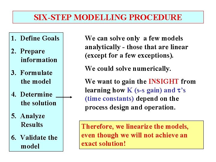
SIX-STEP MODELLING PROCEDURE 1. Define Goals 2. Prepare information 3. Formulate the model 4. Determine the solution 5. Analyze Results 6. Validate the model We can solve only a few models analytically - those that are linear (except for a few exceptions). We could solve numerically. We want to gain the INSIGHT from learning how K (s-s gain) and ’s (time constants) depend on the process design and operation. Therefore, we linearize the models, even though we will not achieve an exact solution!

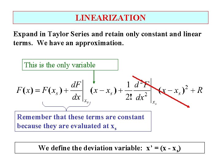
LINEARIZATION Expand in Taylor Series and retain only constant and linear terms. We have an approximation. This is the only variable Remember that these terms are constant because they are evaluated at xs We define the deviation variable: x’ = (x - xs)

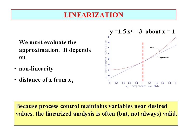
LINEARIZATION y =1. 5 x 2 + 3 about x = 1 We must evaluate the approximation. It depends on • non-linearity • distance of x from xs Because process control maintains variables near desired values, the linearized analysis is often (but, not always) valid.

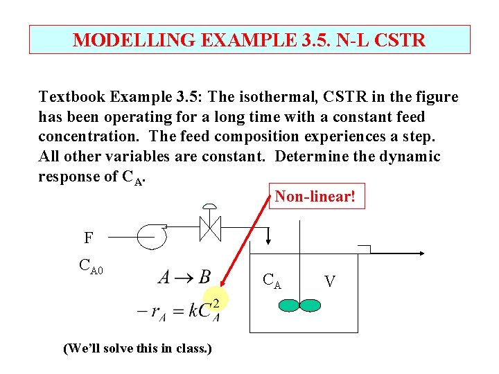
MODELLING EXAMPLE 3. 5. N-L CSTR Textbook Example 3. 5: The isothermal, CSTR in the figure has been operating for a long time with a constant feed concentration. The feed composition experiences a step. All other variables are constant. Determine the dynamic response of CA. Non-linear! F CA 0 (We’ll solve this in class. ) CA V

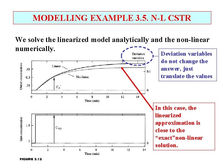
MODELLING EXAMPLE 3. 5. N-L CSTR We solve the linearized model analytically and the non-linear numerically. Deviation variables do not change the answer, just translate the values In this case, the linearized approximation is close to the “exact”non-linear solution.

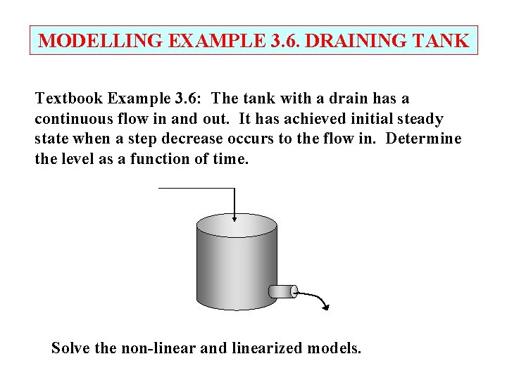
MODELLING EXAMPLE 3. 6. DRAINING TANK Textbook Example 3. 6: The tank with a drain has a continuous flow in and out. It has achieved initial steady state when a step decrease occurs to the flow in. Determine the level as a function of time. Solve the non-linear and linearized models.

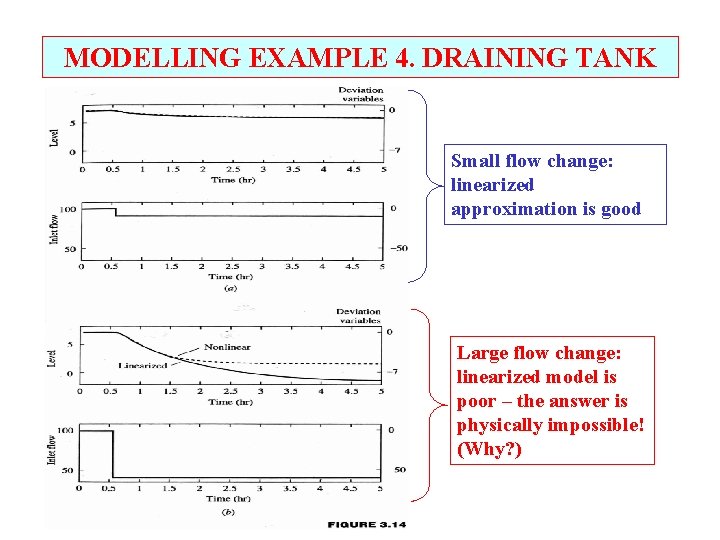
MODELLING EXAMPLE 4. DRAINING TANK Small flow change: linearized approximation is good Large flow change: linearized model is poor – the answer is physically impossible! (Why? )

DYNAMIC MODELLING We learned first-order systems have the same output “shape”. Output is smooth, monotonic curve 1. 6 Maximum slope at “t=0” 1. 4 1. 2 1 63% of steady-state At steady state = K 0. 8 0 20 40 Output changes immediately 60 80 100 120 time 2 inlet concentration Sample response to a step input tank concentration 1. 8 1. 5 = Step in inlet variable 1 0. 5 0 20 40 60 time

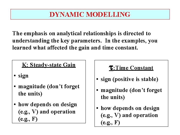
DYNAMIC MODELLING The emphasis on analytical relationships is directed to understanding the key parameters. In the examples, you learned what affected the gain and time constant. K: Steady-state Gain • sign • magnitude (don’t forget the units) • how depends on design (e. g. , V) and operation (e. g. , F) : Time Constant • sign (positive is stable) • magnitude (don’t forget the units) • how depends on design (e. g. , V) and operation (e. g. , F)

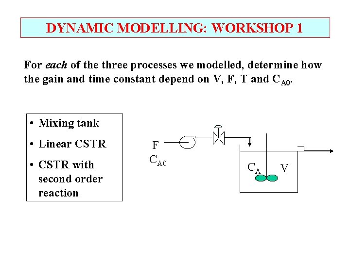
DYNAMIC MODELLING: WORKSHOP 1 For each of the three processes we modelled, determine how the gain and time constant depend on V, F, T and CA 0. • Mixing tank • Linear CSTR • CSTR with second order reaction F CA 0 CA V

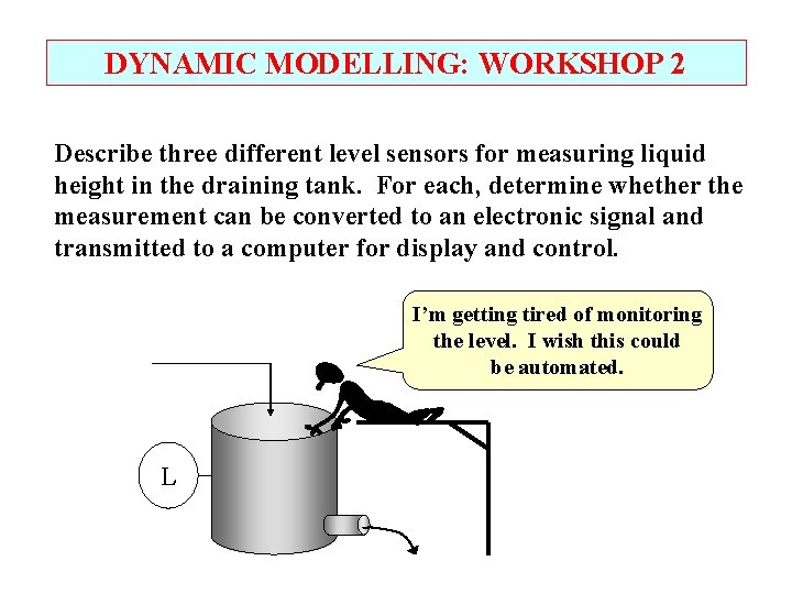
DYNAMIC MODELLING: WORKSHOP 2 Describe three different level sensors for measuring liquid height in the draining tank. For each, determine whether the measurement can be converted to an electronic signal and transmitted to a computer for display and control. I’m getting tired of monitoring the level. I wish this could be automated. L

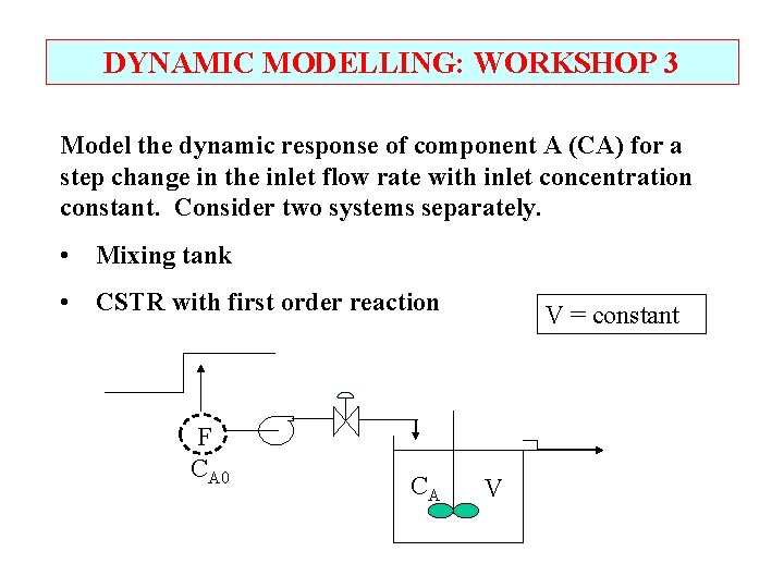
DYNAMIC MODELLING: WORKSHOP 3 Model the dynamic response of component A (CA) for a step change in the inlet flow rate with inlet concentration constant. Consider two systems separately. • Mixing tank • CSTR with first order reaction F CA 0 CA V = constant V

DYNAMIC MODELLING: WORKSHOP 4 The parameters we use in mathematical models are never known exactly. For several models solved in the textbook, evaluate the effect of the solution of errors in parameters. • 20% in reaction rate constant k • 20% in heat transfer coefficient • 5% in flow rate and tank volume How would you consider errors in several parameters in the same problem? Check your responses by simulating using the MATLAB mfiles in the Software Laboratory.

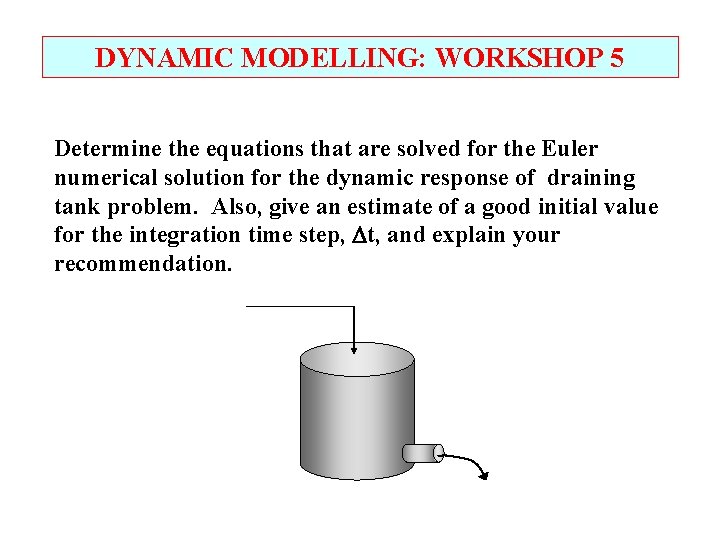
DYNAMIC MODELLING: WORKSHOP 5 Determine the equations that are solved for the Euler numerical solution for the dynamic response of draining tank problem. Also, give an estimate of a good initial value for the integration time step, t, and explain your recommendation.

DYNAMIC MODELLING: WORKSHOP 6 A. Select a topic of interest to you that can be investigated using mathematical modelling and research developments in modelling the topic. For some ideas, see the following. http: //plus. maths. org/content/teacher-packagemathematical-modelling B. Results from mathematical models contain uncertainty. Review the following report and discuss uncertainty in the models that you investigated in Part A above. http: //www. nap. edu/openbook. php? record_id=13395

CHAPTER 3 : MATH. MODELLING How are we doing? • Formulate dynamic models based on fundamental balances • Solve simple first-order linear dynamic models • Determine how key aspects of dynamics depend on process design and operation Lot’s of improvement, but we need some more study! • Read the textbook • Review the notes, especially learning goals and workshop • Try out the self-study suggestions • Naturally, we’ll have an assignment!

CHAPTER 3: LEARNING RESOURCES • SITE PC-EDUCATION WEB - Instrumentation Notes - Interactive Learning Module (Chapter 3) www. pc-education. mcmaster. ca - Tutorials (Chapter 3) - M-files in the Software Laboratory (Chapter 3) • Read the sections on dynamic modelling in previous textbooks - Felder and Rousseau, Fogler, Incropera & Dewitt

CHAPTER 3: SUGGESTIONS FOR SELF-STUDY 1. Discuss why we require that the degrees of freedom for a model must be zero. Are there exceptions? 2. Give examples of constitutive equations from prior chemical engineering courses. For each, describe how we determine the value for the parameter. How accurate is the value? 3. Prepare one question of each type and share with your study group: T/F, multiple choice, and modelling. 4. Using the MATLAB m-files in the Software Laboratory, determine the effect of input step magnitude on linearized model accuracy for the CSTR with second-order reaction.

CHAPTER 3: SUGGESTIONS FOR SELF-STUDY 5. For what combination of physical parameters will a first order dynamic model predict the following? • an oscillatory response to a step input • an output that increases without limit • an output that changes very slowly 6. Prepare a fresh cup of hot coffee or tea. Measure the temperature and record the temperature and time until the temperature approaches ambient. • Plot the data. • Discuss the shape of the temperature plot. • Can you describe it by a response by a key parameter? • Derive a mathematical model and compare with your experimental results