Process Control Designing Process and Control Systems for

Process Control: Designing Process and Control Systems for Dynamic Performance Chapter 4. Modelling and Analysis for Process Control Copyright © Thomas Marlin 2013 The copyright holder provides a royalty-free license for use of this material at non-profit educational institutions

CHAPTER 4 : MODELLING & ANALYSIS FOR PROCESS CONTROL When I complete this chapter, I want to be able to do the following. • Analytically solve linear dynamic models of first and second order • Express dynamic models as transfer functions • Predict important features of dynamic behavior from model without solving

CHAPTER 4 : MODELLING & ANALYSIS FOR PROCESS CONTROL Outline of the lesson. • Laplace transform • Solve linear dynamic models • Transfer function model structure • Qualitative features directly from model • Frequency response • Workshop

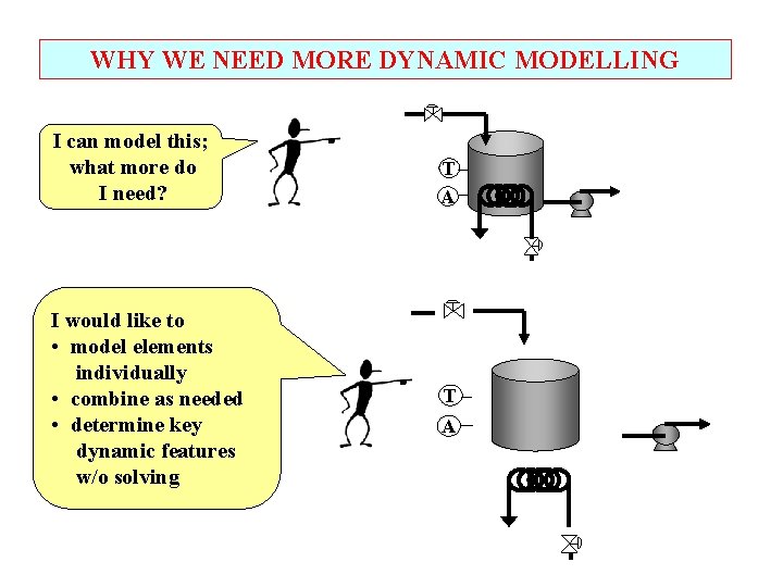
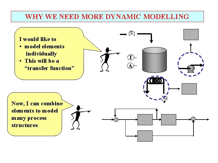
WHY WE NEED MORE DYNAMIC MODELLING I can model this; what more do I need? I would like to • model elements individually • combine as needed • determine key dynamic features w/o solving T A

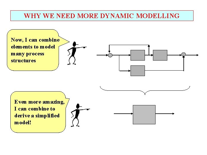
WHY WE NEED MORE DYNAMIC MODELLING I would like to • model elements individually • This will be a “transfer function” Now, I can combine elements to model many process structures T A

WHY WE NEED MORE DYNAMIC MODELLING Now, I can combine elements to model many process structures Even more amazing, I can combine to derive a simplified model!

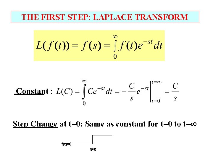
THE FIRST STEP: LAPLACE TRANSFORM Step Change at t=0: Same as constant for t=0 to t= f(t)=0 t=0

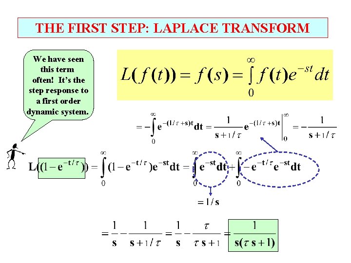
THE FIRST STEP: LAPLACE TRANSFORM We have seen this term often! It’s the step response to a first order dynamic system.

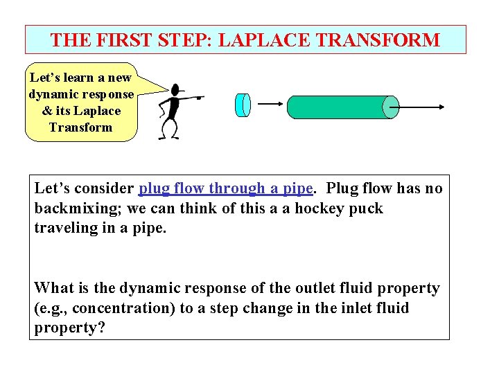
THE FIRST STEP: LAPLACE TRANSFORM Let’s learn a new dynamic response & its Laplace Transform Let’s consider plug flow through a pipe. Plug flow has no backmixing; we can think of this a a hockey puck traveling in a pipe. What is the dynamic response of the outlet fluid property (e. g. , concentration) to a step change in the inlet fluid property?

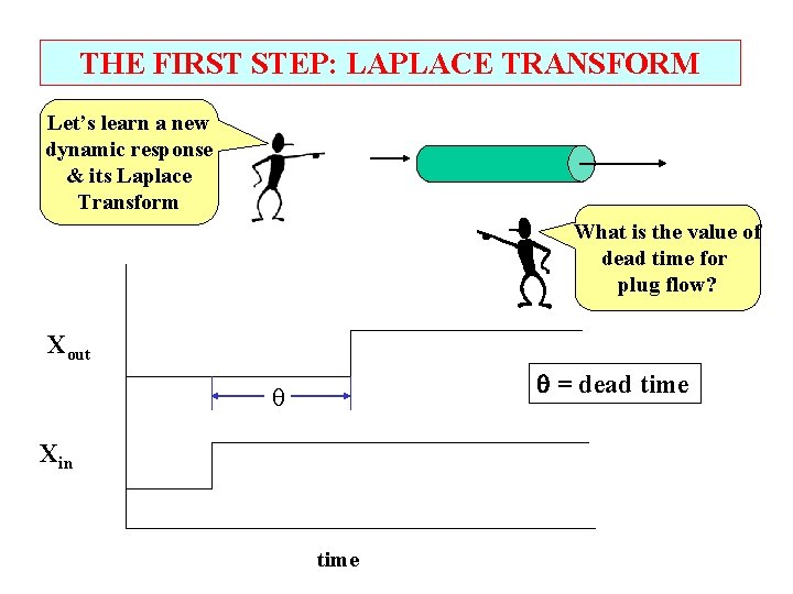
THE FIRST STEP: LAPLACE TRANSFORM Let’s learn a new dynamic response & its Laplace Transform What is the value of dead time for plug flow? Xout = dead time Xin time

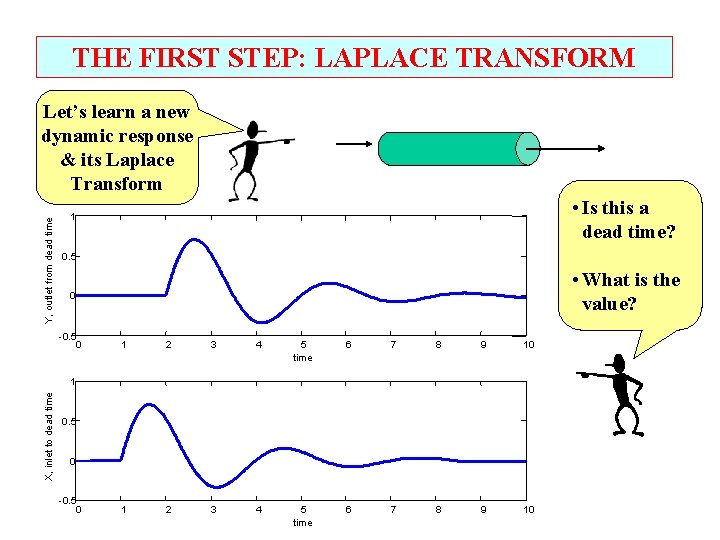
THE FIRST STEP: LAPLACE TRANSFORM Y, outlet from dead time Let’s learn a new dynamic response & its Laplace Transform • Is this a dead time? 1 0. 5 • What is the value? 0 -0. 5 0 1 2 3 4 5 time 6 7 8 9 10 X, inlet to dead time 1 0. 5 0 -0. 5 0

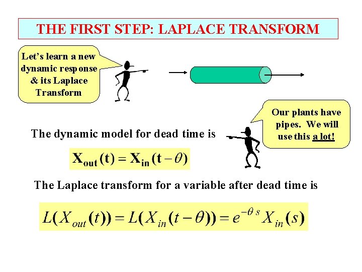
THE FIRST STEP: LAPLACE TRANSFORM Let’s learn a new dynamic response & its Laplace Transform The dynamic model for dead time is Our plants have pipes. We will use this a lot! The Laplace transform for a variable after dead time is

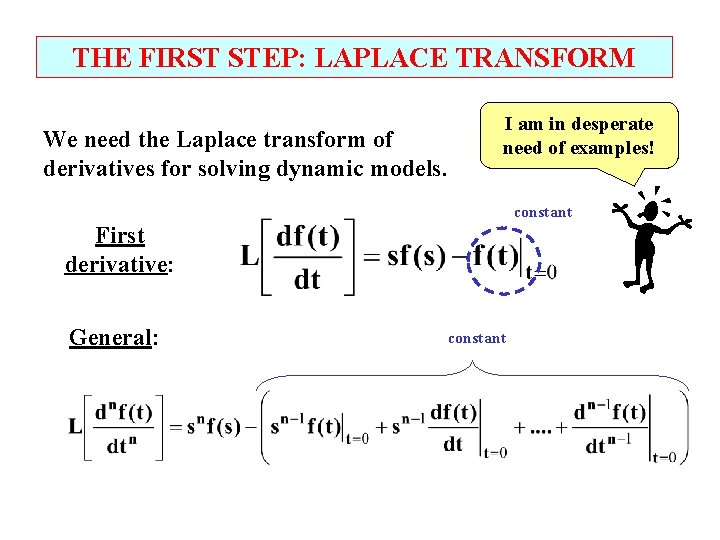
THE FIRST STEP: LAPLACE TRANSFORM We need the Laplace transform of derivatives for solving dynamic models. I am in desperate need of examples! constant First derivative: General: constant

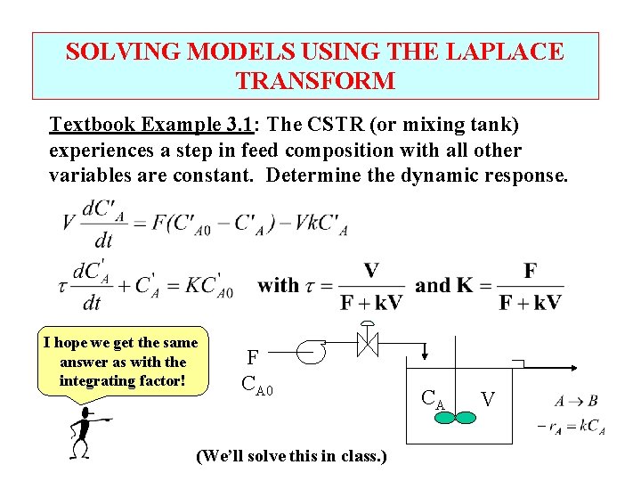
SOLVING MODELS USING THE LAPLACE TRANSFORM Textbook Example 3. 1: The CSTR (or mixing tank) experiences a step in feed composition with all other variables are constant. Determine the dynamic response. I hope we get the same answer as with the integrating factor! F CA 0 (We’ll solve this in class. ) CA V

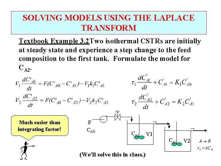
SOLVING MODELS USING THE LAPLACE TRANSFORM Textbook Example 3. 2 Two isothermal CSTRs are initially at steady state and experience a step change to the feed composition to the first tank. Formulate the model for CA 2. Much easier than integrating factor! F CA 0 CA 1 (We’ll solve this in class. ) V 1 CA 2 V 2

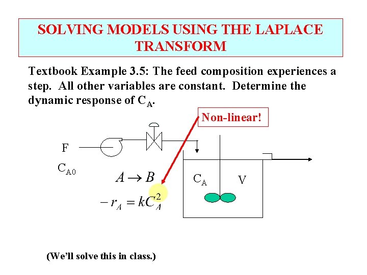
SOLVING MODELS USING THE LAPLACE TRANSFORM Textbook Example 3. 5: The feed composition experiences a step. All other variables are constant. Determine the dynamic response of CA. Non-linear! F CA 0 (We’ll solve this in class. ) CA V

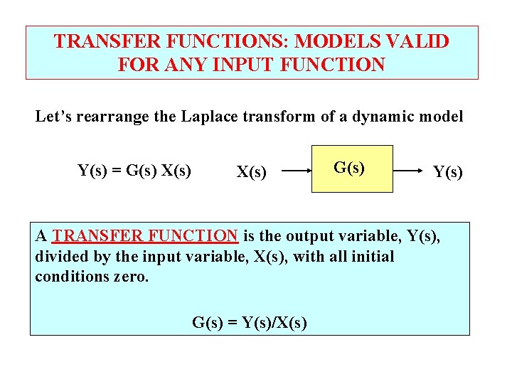
TRANSFER FUNCTIONS: MODELS VALID FOR ANY INPUT FUNCTION Let’s rearrange the Laplace transform of a dynamic model Y(s) = G(s) X(s) G(s) Y(s) A TRANSFER FUNCTION is the output variable, Y(s), divided by the input variable, X(s), with all initial conditions zero. G(s) = Y(s)/X(s)

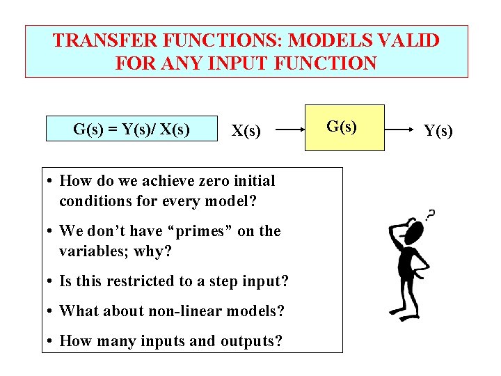
TRANSFER FUNCTIONS: MODELS VALID FOR ANY INPUT FUNCTION G(s) = Y(s)/ X(s) • How do we achieve zero initial conditions for every model? • We don’t have “primes” on the variables; why? • Is this restricted to a step input? • What about non-linear models? • How many inputs and outputs? G(s) Y(s)

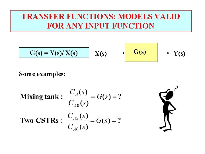
TRANSFER FUNCTIONS: MODELS VALID FOR ANY INPUT FUNCTION G(s) = Y(s)/ X(s) Some examples: X(s) G(s) Y(s)

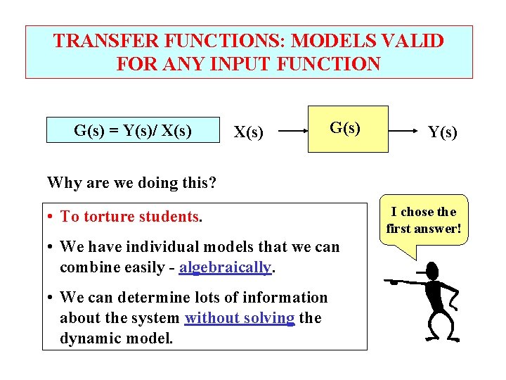
TRANSFER FUNCTIONS: MODELS VALID FOR ANY INPUT FUNCTION G(s) = Y(s)/ X(s) G(s) Y(s) Why are we doing this? • To torture students. • We have individual models that we can combine easily - algebraically. • We can determine lots of information about the system without solving the dynamic model. I chose the first answer!

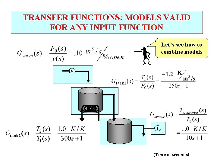
TRANSFER FUNCTIONS: MODELS VALID FOR ANY INPUT FUNCTION Let’s see how to combine models T (Time in seconds)

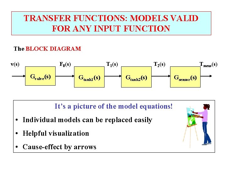
TRANSFER FUNCTIONS: MODELS VALID FOR ANY INPUT FUNCTION The BLOCK DIAGRAM v(s) F 0(s) Gvalve(s) T 1(s) Gtank 1(s) T 2(s) Gtank 2(s) It’s a picture of the model equations! • Individual models can be replaced easily • Helpful visualization • Cause-effect by arrows Tmeas(s) Gsensor(s)

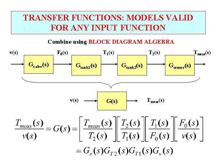
TRANSFER FUNCTIONS: MODELS VALID FOR ANY INPUT FUNCTION Combine using BLOCK DIAGRAM ALGEBRA v(s) F 0(s) Gvalve(s) T 1(s) Gtank 1(s) v(s) T 2(s) Gtank 2(s) G(s) Tmeas(s) Gsensor(s) Tmeas(s)

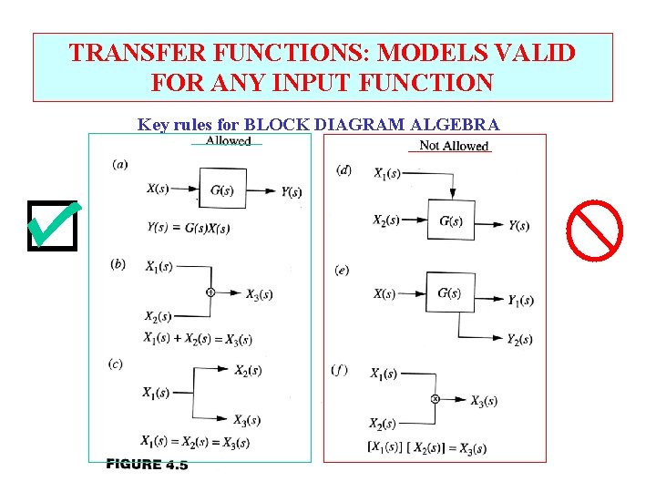
TRANSFER FUNCTIONS: MODELS VALID FOR ANY INPUT FUNCTION Key rules for BLOCK DIAGRAM ALGEBRA

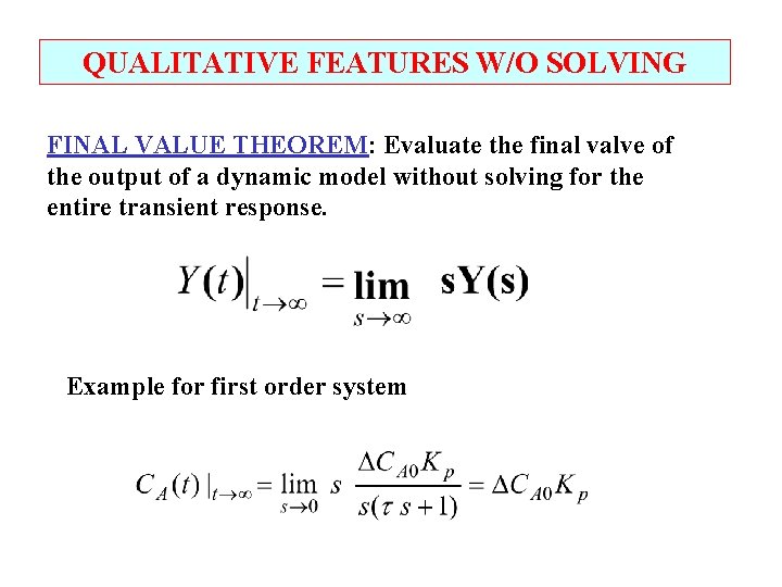
QUALITATIVE FEATURES W/O SOLVING FINAL VALUE THEOREM: Evaluate the final valve of the output of a dynamic model without solving for the entire transient response. Example for first order system

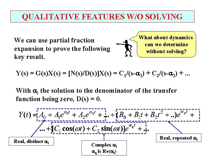
QUALITATIVE FEATURES W/O SOLVING We can use partial fraction expansion to prove the following key result. What about dynamics can we determine without solving? Y(s) = G(s)X(s) = [N(s)/D(s)]X(s) = C 1/(s- 1) + C 2/(s- 2) +. . . With i the solution to the denominator of the transfer function being zero, D(s) = 0. Real, distinct i Complex i q is Re( i) Real, repeated i

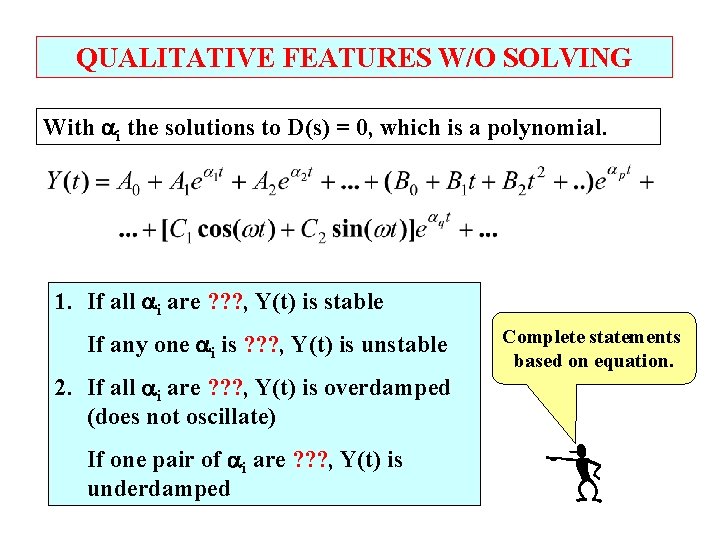
QUALITATIVE FEATURES W/O SOLVING With i the solutions to D(s) = 0, which is a polynomial. 1. If all i are ? ? ? , Y(t) is stable If any one i is ? ? ? , Y(t) is unstable 2. If all i are ? ? ? , Y(t) is overdamped (does not oscillate) If one pair of i are ? ? ? , Y(t) is underdamped Complete statements based on equation.

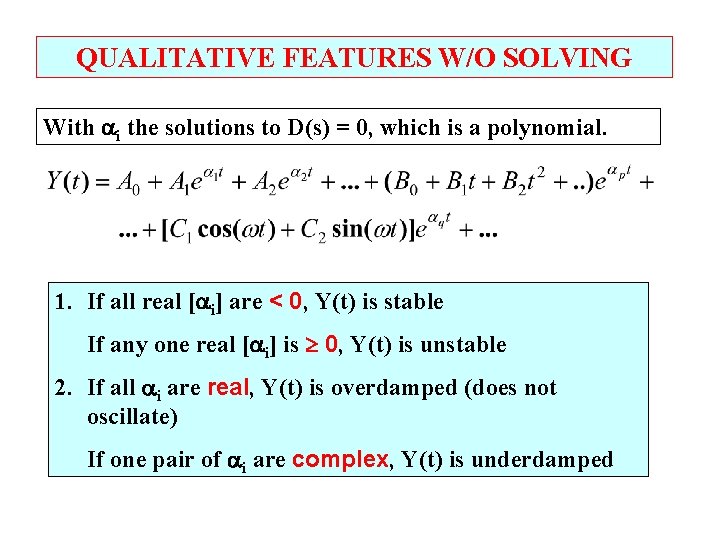
QUALITATIVE FEATURES W/O SOLVING With i the solutions to D(s) = 0, which is a polynomial. 1. If all real [ i] are < 0, Y(t) is stable If any one real [ i] is 0, Y(t) is unstable 2. If all i are real, Y(t) is overdamped (does not oscillate) If one pair of i are complex, Y(t) is underdamped

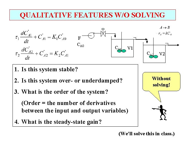
QUALITATIVE FEATURES W/O SOLVING F CA 0 CA 1 V 1 CA 2 V 2 1. Is this system stable? 2. Is this system over- or underdamped? Without solving! 3. What is the order of the system? (Order = the number of derivatives between the input and output variables) 4. What is the steady-state gain? (We’ll solve this in class. )

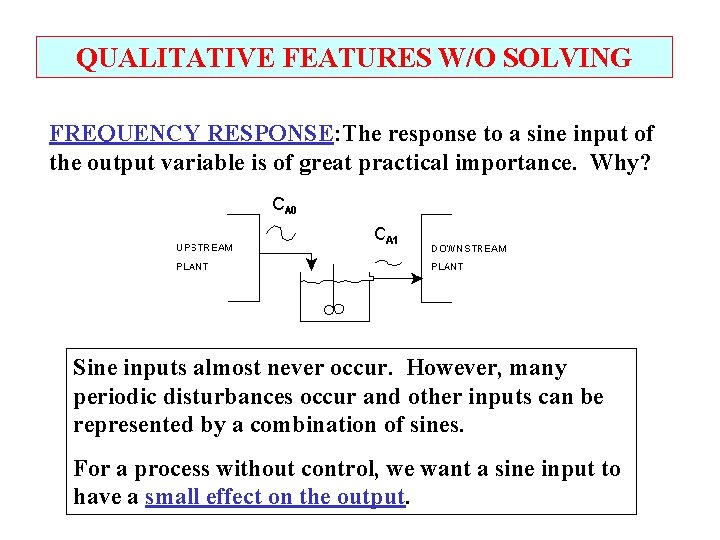
QUALITATIVE FEATURES W/O SOLVING FREQUENCY RESPONSE: The response to a sine input of the output variable is of great practical importance. Why? Sine inputs almost never occur. However, many periodic disturbances occur and other inputs can be represented by a combination of sines. For a process without control, we want a sine input to have a small effect on the output.

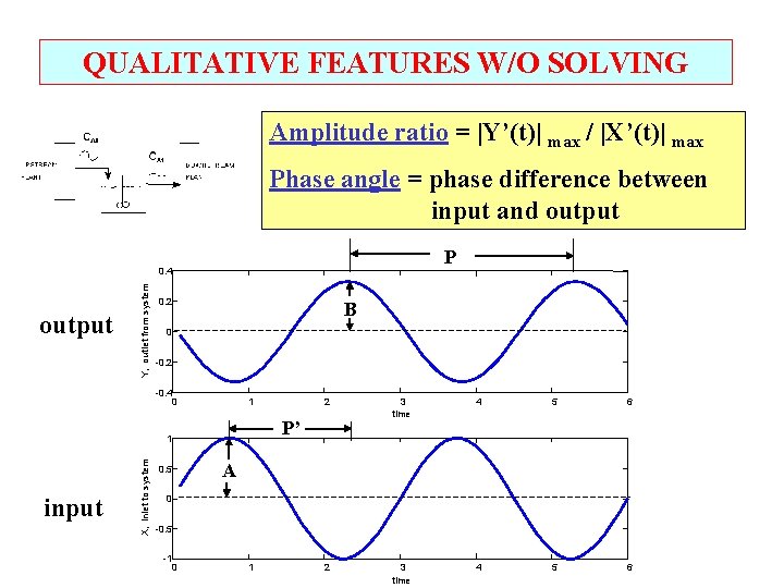
QUALITATIVE FEATURES W/O SOLVING Amplitude ratio = |Y’(t)| max / |X’(t)| max Phase angle = phase difference between input and output P output Y, outlet from system 0. 4 0. 2 B 0 -0. 2 -0. 4 0 1 X, inlet to system 3 time 4 5 6 2 3 time 4 5 6 P’ 1 input 2 A 0. 5 0 -0. 5 -1 0 1

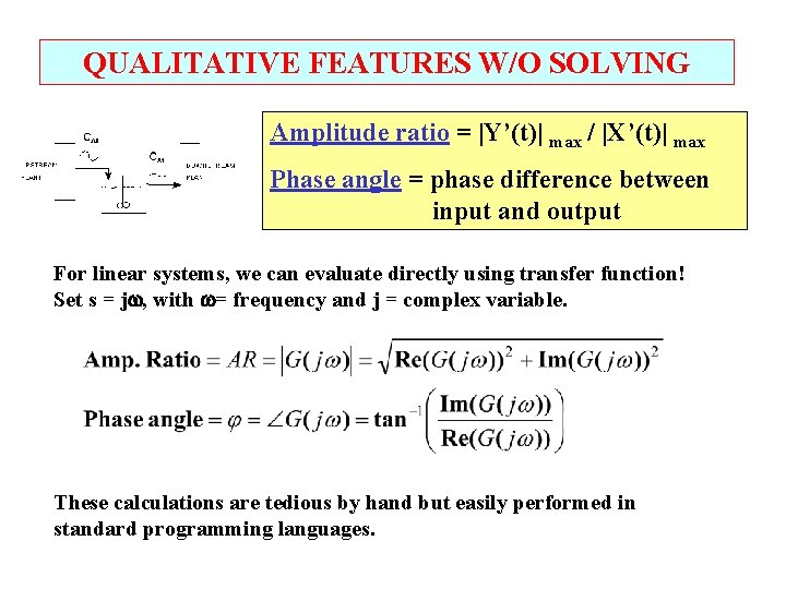
QUALITATIVE FEATURES W/O SOLVING Amplitude ratio = |Y’(t)| max / |X’(t)| max Phase angle = phase difference between input and output For linear systems, we can evaluate directly using transfer function! Set s = j , with = frequency and j = complex variable. These calculations are tedious by hand but easily performed in standard programming languages.

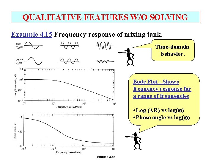
QUALITATIVE FEATURES W/O SOLVING Example 4. 15 Frequency response of mixing tank. Time-domain behavior. Bode Plot - Shows frequency response for a range of frequencies • Log (AR) vs log( ) • Phase angle vs log( )

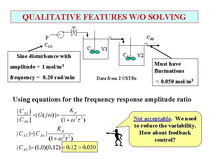
QUALITATIVE FEATURES W/O SOLVING F CA 0 Sine disturbance with CA 2 CA 1 V 1 CA 2 V 2 Must have fluctuations amplitude = 1 mol/m 3 frequency = 0. 20 rad/min Data from 2 CSTRs < 0. 050 mol/m 3 Using equations for the frequency response amplitude ratio Not acceptable. We need to reduce the variability. How about feedback control?

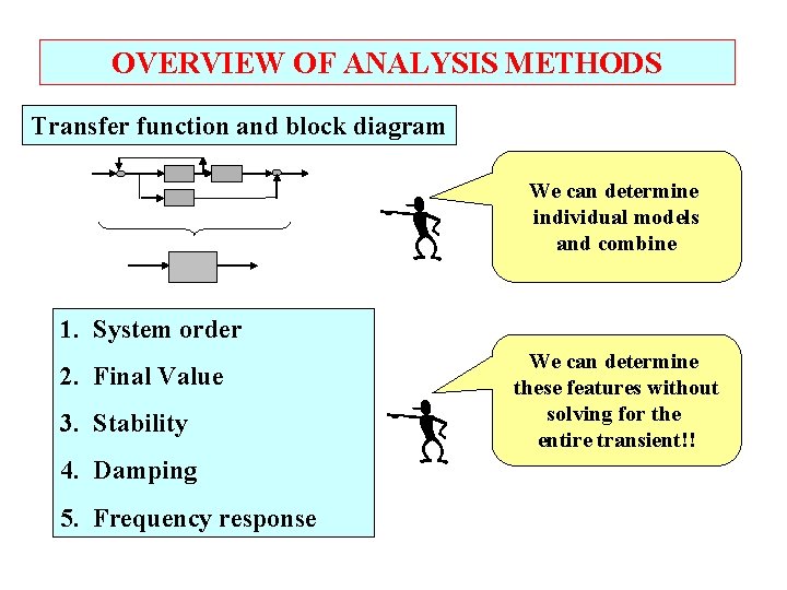
OVERVIEW OF ANALYSIS METHODS Transfer function and block diagram We can determine individual models and combine 1. System order 2. Final Value 3. Stability 4. Damping 5. Frequency response We can determine these features without solving for the entire transient!!

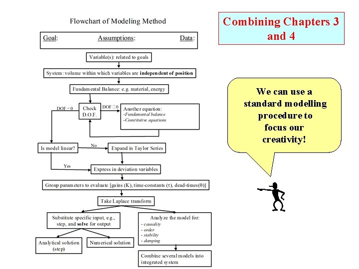
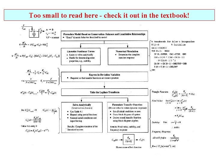
Combining Chapters 3 and 4 We can use a standard modelling procedure to focus our creativity!

Too small to read here - check it out in the textbook!

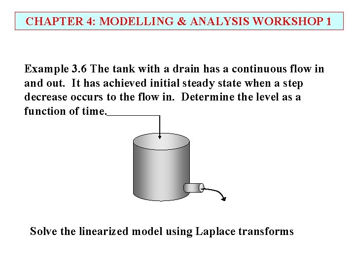
CHAPTER 4: MODELLING & ANALYSIS WORKSHOP 1 Example 3. 6 The tank with a drain has a continuous flow in and out. It has achieved initial steady state when a step decrease occurs to the flow in. Determine the level as a function of time. Solve the linearized model using Laplace transforms

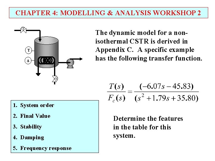
CHAPTER 4: MODELLING & ANALYSIS WORKSHOP 2 T A The dynamic model for a nonisothermal CSTR is derived in Appendix C. A specific example has the following transfer function. 1. System order 2. Final Value 3. Stability 4. Damping 5. Frequency response Determine the features in the table for this system.

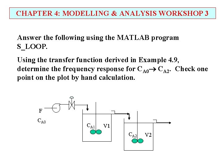
CHAPTER 4: MODELLING & ANALYSIS WORKSHOP 3 Answer the following using the MATLAB program S_LOOP. Using the transfer function derived in Example 4. 9, determine the frequency response for CA 0 CA 2. Check one point on the plot by hand calculation. F CA 0 CA 1 V 1 CA 2 V 2

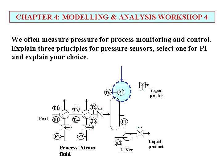
CHAPTER 4: MODELLING & ANALYSIS WORKSHOP 4 We often measure pressure for process monitoring and control. Explain three principles for pressure sensors, select one for P 1 and explain your choice. T 6 Feed T 1 T 2 T 5 F 1 T 4 T 3 F 2 P 1 L 1 F 3 Process Steam fluid Vapor product A 1 L. Key Liquid product

CHAPTER 4 : MODELLING & ANALYSIS FOR PROCESS CONTROL When I complete this chapter, I want to be able to do the following. • Analytically solve linear dynamic models of first and second order • Express dynamic models as transfer functions • Predict important features of dynamic behavior from model without solving Lot’s of improvement, but we need some more study! • Read the textbook • Review the notes, especially learning goals and workshop • Try out the self-study suggestions • Naturally, we’ll have an assignment!

LEARNING RESOURCES • SITE PC-EDUCATION WEB - Instrumentation Notes - Interactive Learning Module (Chapter 4) www. pc-education. mcmaster. ca - Tutorials (Chapter 4) • Software Laboratory - S_LOOP program

SUGGESTIONS FOR SELF-STUDY 1. Why are variables expressed as deviation variables when we develop transfer functions? 2. Discuss the difference between a second order reaction and a second order dynamic model. 3. For a sine input to a process, is the output a sine for a a. Linear plant? b. Non-linear plant? 4. Is the amplitude ratio of a plant always equal to or greater than the steady-state gain?

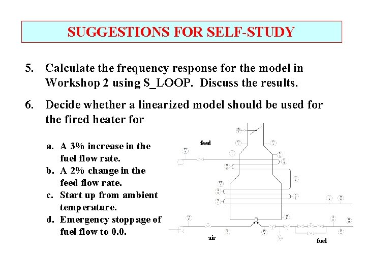
SUGGESTIONS FOR SELF-STUDY 5. Calculate the frequency response for the model in Workshop 2 using S_LOOP. Discuss the results. 6. Decide whether a linearized model should be used for the fired heater for a. A 3% increase in the fuel flow rate. b. A 2% change in the feed flow rate. c. Start up from ambient temperature. d. Emergency stoppage of fuel flow to 0. 0. feed air fuel