Process Control Designing Process and Control Systems for

Process Control: Designing Process and Control Systems for Dynamic Performance Chapter 10. Stability and Tuning Copyright © Thomas Marlin 2013 The copyright holder provides a royalty-free license for use of this material at non-profit educational institutions

CHAPTER 10: STABILITY &TUNING When I complete this chapter, I want to be able to do the following. • Determine the stability of a process without control • Determine the stability of a closed-loop feedback control system • Use these approaches to learn how dead time affects stability.

CHAPTER 10: STABILITY &TUNING Outline of the lesson. • Define stability • Review determining the roots of the characteristic equation • Introduce the Bode stability method • Apply to determine some general trends in feedback systems

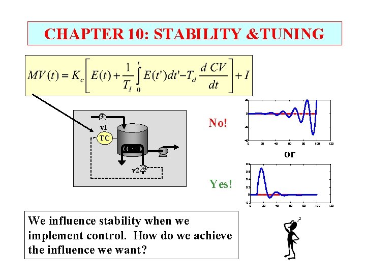
CHAPTER 10: STABILITY &TUNING 20 0 No! v 1 TC -20 -40 0 20 40 60 80 100 120 or 0. 8 v 2 0. 6 Yes! 0. 4 0. 2 0 -0. 2 0 We influence stability when we implement control. How do we achieve the influence we want? 20 40 60

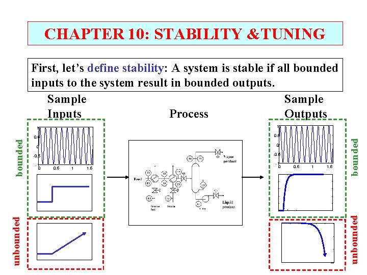
CHAPTER 10: STABILITY &TUNING 1 0. 5 0 0 -0. 5 -1 0 0. 5 1 1. 5 bounded 1 unbounded First, let’s define stability: A system is stable if all bounded inputs to the system result in bounded outputs. Sample Inputs Process Outputs

CHAPTER 10: STABILITY &TUNING G(s) = Y(s)/X(s) Y(s) = [N(s)/D(s)] X(s) Let’s review how we determine the stability of a model. With i the solution to the denominator of the transfer function being zero, D(s) = 0 giving s = 1, 2 , i. . Real, distinct i Complex i If all i are ? ? ? , Y(t) is stable If any one i is ? ? ? , Y(t) is unstable Real, repeated i Class exercise

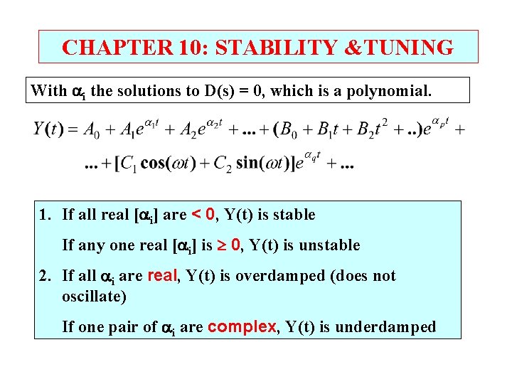
CHAPTER 10: STABILITY &TUNING With i the solutions to D(s) = 0, which is a polynomial. 1. If all real [ i] are < 0, Y(t) is stable If any one real [ i] is 0, Y(t) is unstable 2. If all i are real, Y(t) is overdamped (does not oscillate) If one pair of i are complex, Y(t) is underdamped

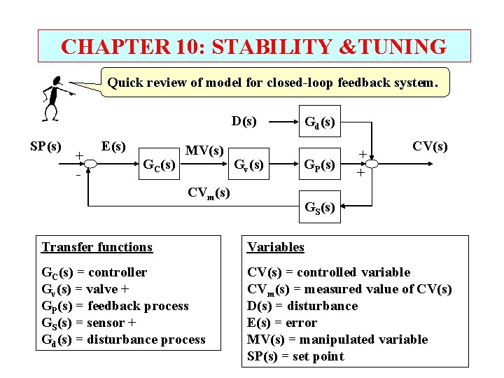
CHAPTER 10: STABILITY &TUNING Quick review of model for closed-loop feedback system. D(s) SP(s) + - E(s) GC(s) MV(s) CVm(s) Gv(s) Gd(s) GP(s) + + CV(s) GS(s) Transfer functions Variables GC(s) = controller Gv(s) = valve + GP(s) = feedback process GS(s) = sensor + Gd(s) = disturbance process CV(s) = controlled variable CVm(s) = measured value of CV(s) D(s) = disturbance E(s) = error MV(s) = manipulated variable SP(s) = set point

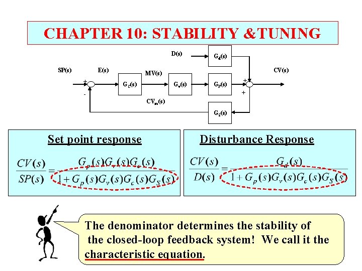
CHAPTER 10: STABILITY &TUNING D(s) SP(s) E(s) + Gd(s) CV(s) MV(s) GC(s) Gv(s) GP(s) + + CVm(s) GS(s) Set point response Disturbance Response The denominator determines the stability of the closed-loop feedback system! We call it the characteristic equation.

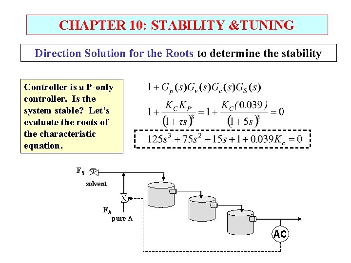
CHAPTER 10: STABILITY &TUNING Direction Solution for the Roots to determine the stability Controller is a P-only controller. Is the system stable? Let’s evaluate the roots of the characteristic equation. FS solvent FA pure A AC

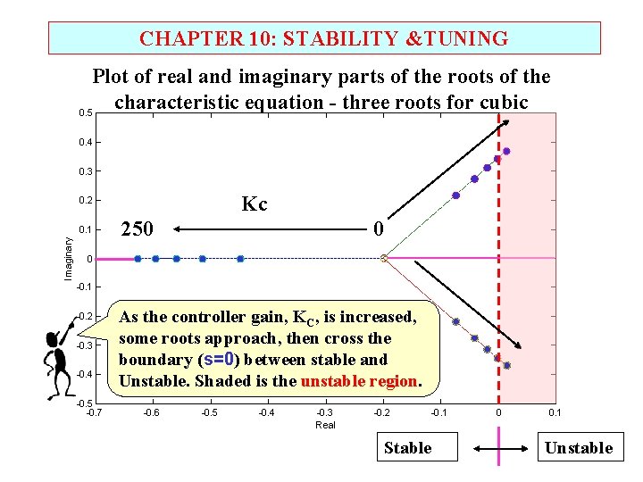
CHAPTER 10: STABILITY &TUNING Plot of real and imaginary parts of the roots of the characteristic equation - three roots for cubic 0. 5 0. 4 0. 3 Kc 0. 2 Imaginary 0. 1 250 0 0 -0. 1 -0. 2 -0. 3 -0. 4 -0. 5 -0. 7 As the controller gain, KC, is increased, some roots approach, then cross the boundary (s=0) between stable and Unstable. Shaded is the unstable region. -0. 6 -0. 5 -0. 4 -0. 3 Real -0. 2 -0. 1 Stable 0 0. 1 Unstable

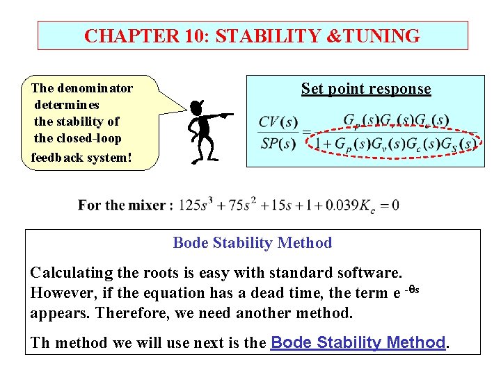
CHAPTER 10: STABILITY &TUNING The denominator determines the stability of the closed-loop feedback system! Set point response Bode Stability Method Calculating the roots is easy with standard software. However, if the equation has a dead time, the term e - s appears. Therefore, we need another method. Th method we will use next is the Bode Stability Method.

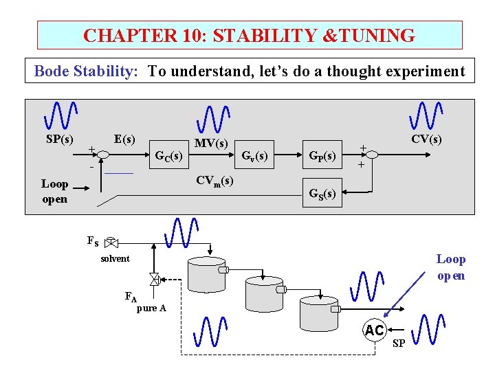
CHAPTER 10: STABILITY &TUNING Bode Stability: To understand, let’s do a thought experiment SP(s) + - E(s) GC(s) MV(s) CVm(s) Loop open Gv(s) GP(s) CV(s) + + GS(s) FS Loop open solvent FA pure A AC SP

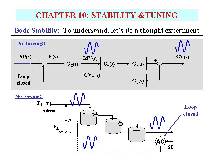
CHAPTER 10: STABILITY &TUNING Bode Stability: To understand, let’s do a thought experiment No forcing!! SP(s) + - E(s) GC(s) MV(s) CVm(s) Loop closed Gv(s) GP(s) CV(s) + + GS(s) No forcing!! FS Loop closed solvent FA pure A AC SP

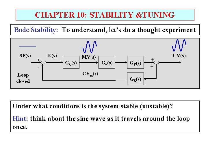
CHAPTER 10: STABILITY &TUNING Bode Stability: To understand, let’s do a thought experiment SP(s) Loop closed + - E(s) GC(s) MV(s) CVm(s) Gv(s) GP(s) + + CV(s) GS(s) Under what conditions is the system stable (unstable)? Hint: think about the sine wave as it travels around the loop once.

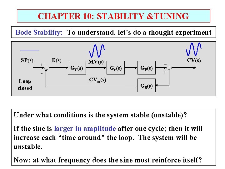
CHAPTER 10: STABILITY &TUNING Bode Stability: To understand, let’s do a thought experiment SP(s) Loop closed + - E(s) GC(s) MV(s) CVm(s) Gv(s) GP(s) + + CV(s) GS(s) Under what conditions is the system stable (unstable)? If the sine is larger in amplitude after one cycle; then it will increase each “time around” the loop. The system will be unstable. Now: at what frequency does the sine most reinforce itself?

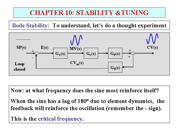
CHAPTER 10: STABILITY &TUNING Bode Stability: To understand, let’s do a thought experiment SP(s) Loop closed + - E(s) GC(s) MV(s) CVm(s) Gv(s) GP(s) + + CV(s) GS(s) Now: at what frequency does the sine most reinforce itself? When the sine has a lag of 180° due to element dynamics, the feedback will reinforce the oscillation (remember the - sign). This is the critical frequency.

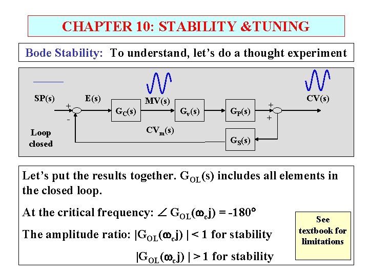
CHAPTER 10: STABILITY &TUNING Bode Stability: To understand, let’s do a thought experiment SP(s) Loop closed + - E(s) GC(s) MV(s) CVm(s) Gv(s) GP(s) + + CV(s) GS(s) Let’s put the results together. GOL(s) includes all elements in the closed loop. At the critical frequency: GOL( cj) = -180 The amplitude ratio: |GOL( cj) | < 1 for stability |GOL( cj) | > 1 for stability See textbook for limitations

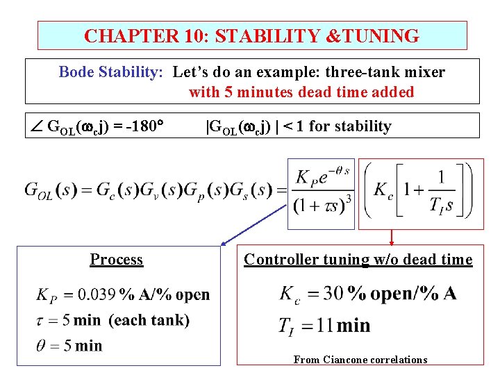
CHAPTER 10: STABILITY &TUNING Bode Stability: Let’s do an example: three-tank mixer with 5 minutes dead time added GOL( cj) = -180 Process |GOL( cj) | < 1 for stability Controller tuning w/o dead time From Ciancone correlations

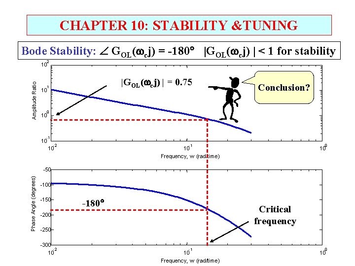
CHAPTER 10: STABILITY &TUNING Bode Stability: GOL( cj) = -180 |GOL( cj) | < 1 for stability 2 Amplitude Ratio 10 |GOL( cj) | = 0. 75 1 10 Conclusion? 0 10 -1 10 -2 -1 10 0 10 Frequency, w (rad/time) 10 Phase Angle (degrees) -50 -100 -150 -180 Critical frequency -200 -250 -300 -2 10 -1 10 Frequency, w (rad/time) 0 10

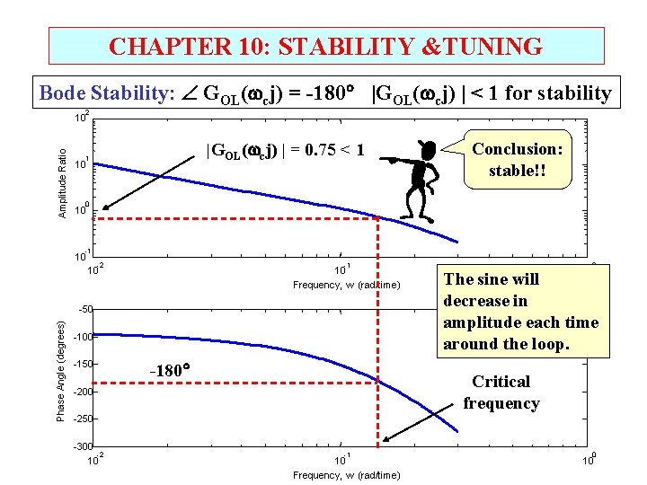
CHAPTER 10: STABILITY &TUNING Bode Stability: GOL( cj) = -180 |GOL( cj) | < 1 for stability 2 Amplitude Ratio 10 |GOL( cj) | = 0. 75 < 1 1 10 Conclusion: stable!! 0 10 -1 10 -2 -1 10 10 Frequency, w (rad/time) Phase Angle (degrees) -50 -100 -150 -180 0 10 The sine will decrease in amplitude each time around the loop. Critical frequency -200 -250 -300 -2 10 -1 10 Frequency, w (rad/time) 0 10

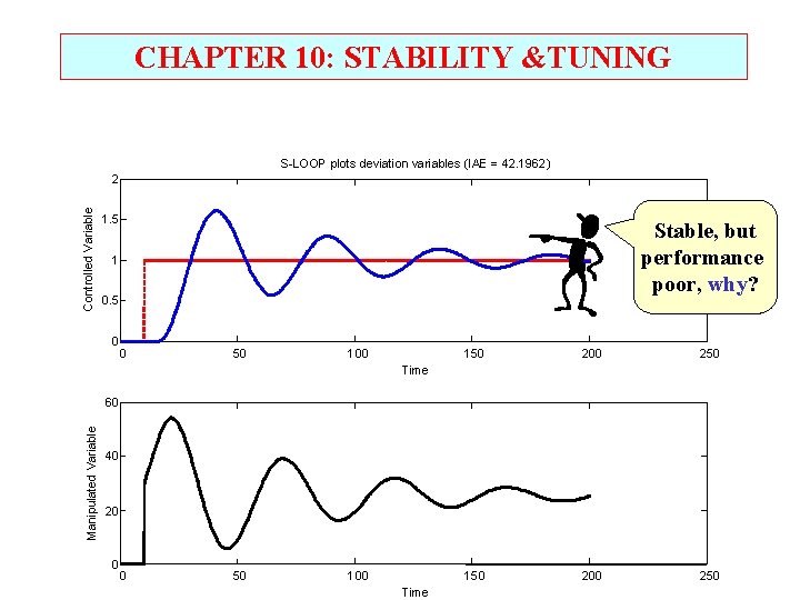
CHAPTER 10: STABILITY &TUNING S-LOOP plots deviation variables (IAE = 42. 1962) Controlled Variable 2 1. 5 Stable, but performance poor, why? 1 0. 5 0 0 50 100 150 200 250 Time Manipulated Variable 60 40 20 0 0 50 100 Time

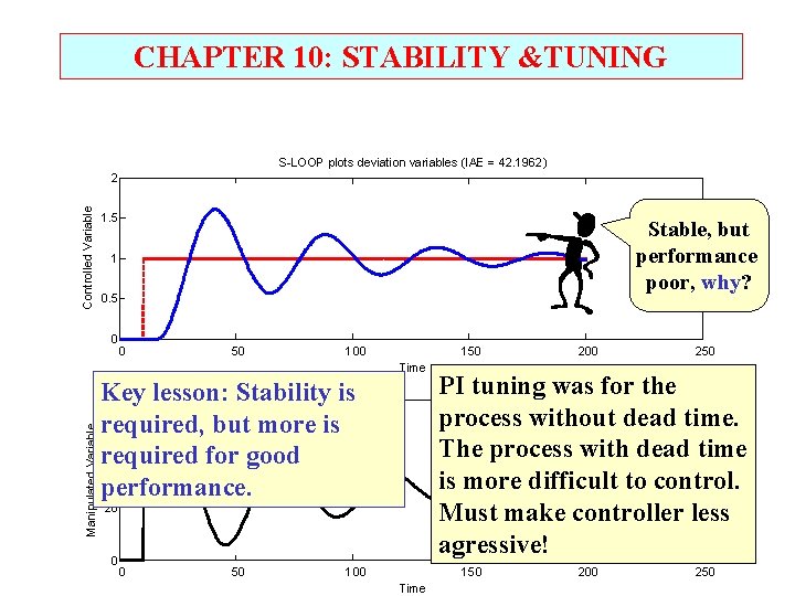
CHAPTER 10: STABILITY &TUNING S-LOOP plots deviation variables (IAE = 42. 1962) Controlled Variable 2 1. 5 Stable, but performance poor, why? 1 0. 5 0 0 50 100 150 Manipulated Variable Time Key lesson: Stability is 60 required, but more is 40 required for good performance. 20 0 0 50 100 250 PI tuning was for the process without dead time. The process with dead time is more difficult to control. Must make controller less agressive! 150 Time 200 250

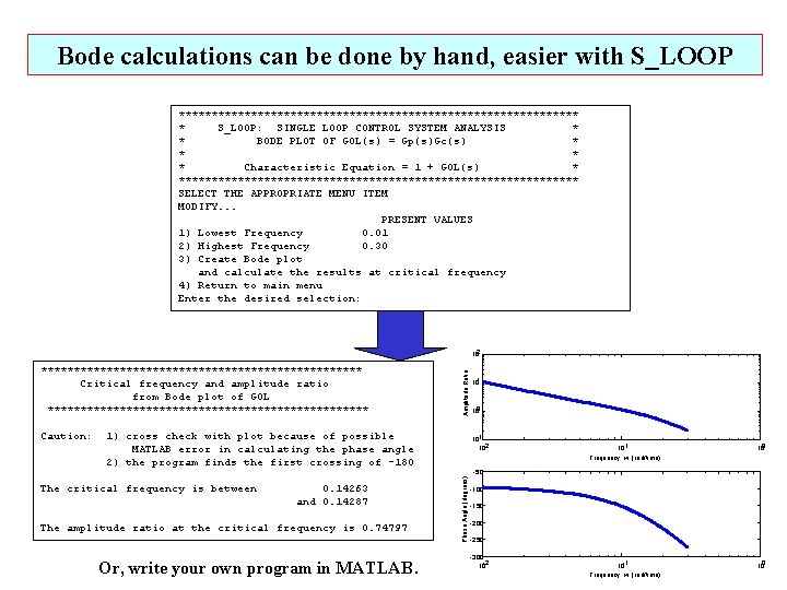
Bode calculations can be done by hand, easier with S_LOOP ******************************* * S_LOOP: SINGLE LOOP CONTROL SYSTEM ANALYSIS * * BODE PLOT OF GOL(s) = Gp(s)Gc(s) * * Characteristic Equation = 1 + GOL(s) * ******************************* SELECT THE APPROPRIATE MENU ITEM MODIFY. . . PRESENT VALUES 1) Lowest Frequency 0. 01 2) Highest Frequency 0. 30 3) Create Bode plot and calculate the results at critical frequency 4) Return to main menu Enter the desired selection: ************************* Critical frequency and amplitude ratio from Bode plot of GOL ************************* 1) cross check with plot because of possible MATLAB error in calculating the phase angle 2) the program finds the first crossing of -180 The critical frequency is between 0. 14263 and 0. 14287 The amplitude ratio at the critical frequency is 0. 74797 Or, write your own program in MATLAB. 101 100 10 -1 10 -2 10 -1 Frequency, w (rad/time) 100 -50 Phase Angle (degrees) Caution: Amplitude Ratio 102 -100 -150 -200 -250 -300 10 -2

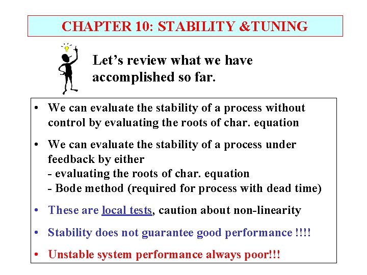
CHAPTER 10: STABILITY &TUNING Let’s review what we have accomplished so far. • We can evaluate the stability of a process without control by evaluating the roots of char. equation • We can evaluate the stability of a process under feedback by either - evaluating the roots of char. equation - Bode method (required for process with dead time) • These are local tests, caution about non-linearity • Stability does not guarantee good performance !!!! • Unstable system performance always poor!!!

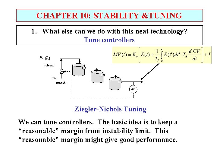
CHAPTER 10: STABILITY &TUNING 1. What else can we do with this neat technology? Tune controllers FS solvent FA pure A AC Ziegler-Nichols Tuning We can tune controllers. The basic idea is to keep a “reasonable” margin from instability limit. This “reasonable” margin might give good performance.

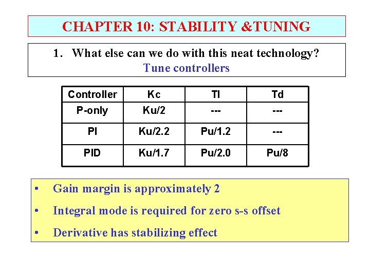
CHAPTER 10: STABILITY &TUNING 1. What else can we do with this neat technology? Tune controllers Controller Kc TI Td P-only Ku/2 --- PI Ku/2. 2 Pu/1. 2 --- PID Ku/1. 7 Pu/2. 0 Pu/8 • Gain margin is approximately 2 • Integral mode is required for zero s-s offset • Derivative has stabilizing effect

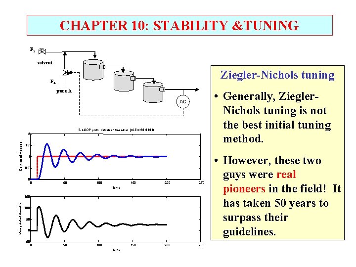
CHAPTER 10: STABILITY &TUNING FS solvent Ziegler-Nichols tuning FA pure A • Generally, Ziegler. Nichols tuning is not the best initial tuning method. AC S-LOOP plots deviation variables (IAE = 23. 3131) Controlled Variable 2 1. 5 1 0. 5 0 0 50 100 150 200 250 Time Manipulated Variable 150 100 50 0 -50 0 50 100 Time • However, these two guys were real pioneers in the field! It has taken 50 years to surpass their guidelines.

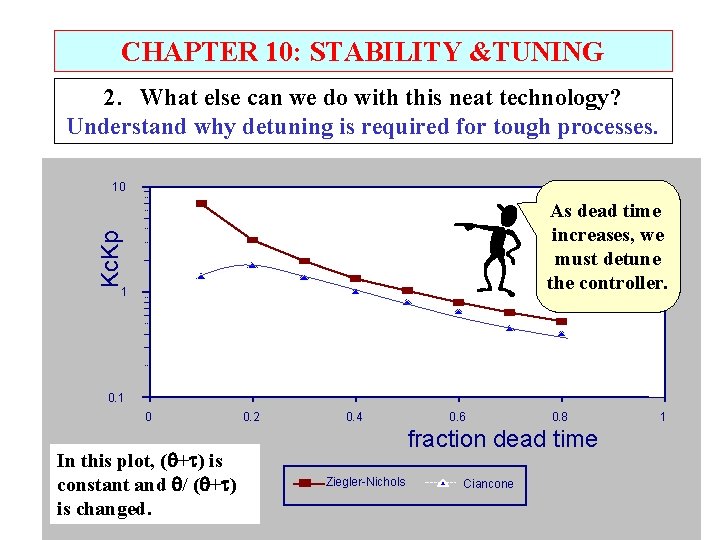
CHAPTER 10: STABILITY &TUNING 2. What else can we do with this neat technology? Understand why detuning is required for tough processes. 10 Kc. Kp As dead time increases, we must detune the controller. 1 0 In this plot, ( + ) is constant and / ( + ) is changed. 0. 2 0. 4 0. 6 0. 8 fraction dead time Ziegler-Nichols Ciancone 1

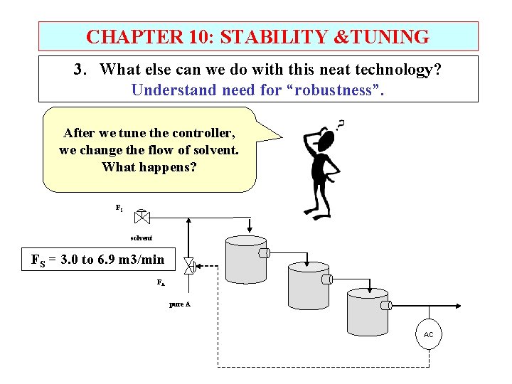
CHAPTER 10: STABILITY &TUNING 3. What else can we do with this neat technology? Understand need for “robustness”. After we tune the controller, we change the flow of solvent. What happens? FS solvent FS = 3. 0 to 6. 9 m 3/min FA pure A AC

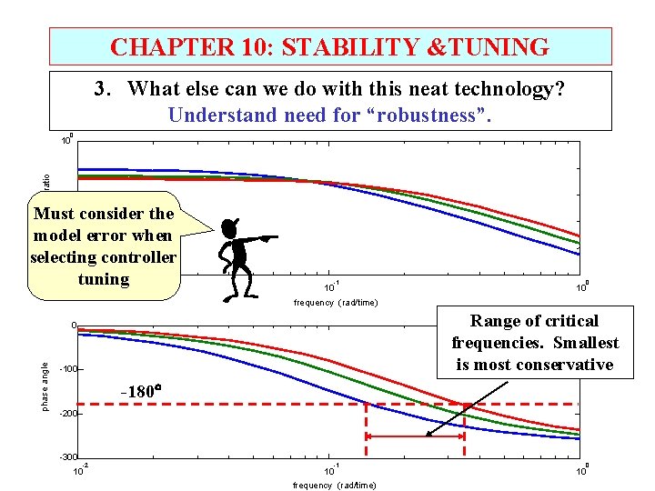
CHAPTER 10: STABILITY &TUNING 3. What else can we do with this neat technology? Understand need for “robustness”. 0 amplitude ratio 10 Must consider the model error when selecting controller 10 tuning 10 -5 -2 -1 10 0 10 frequency (rad/time) Range of critical frequencies. Smallest is most conservative phase angle 0 -100 -180 -200 -300 -2 10 -1 10 frequency (rad/time) 0 10

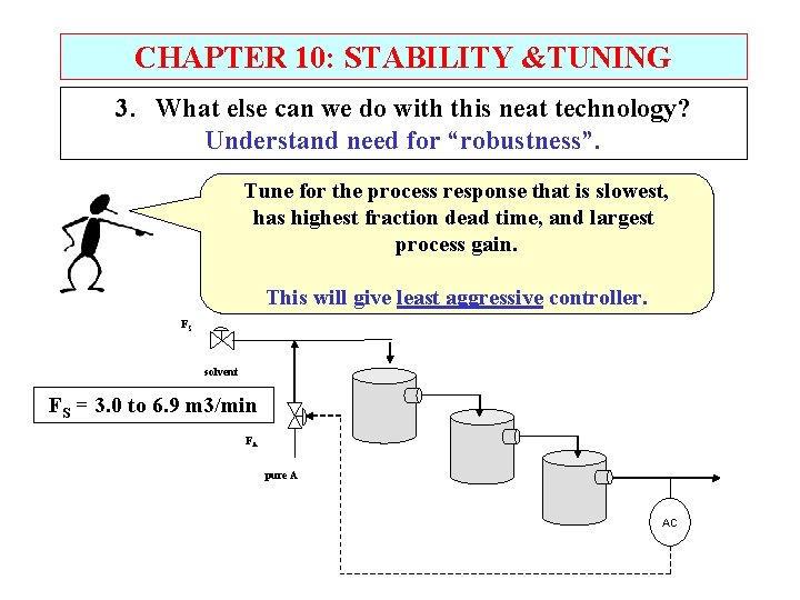
CHAPTER 10: STABILITY &TUNING 3. What else can we do with this neat technology? Understand need for “robustness”. Tune for the process response that is slowest, has highest fraction dead time, and largest process gain. This will give least aggressive controller. FS solvent FS = 3. 0 to 6. 9 m 3/min FA pure A AC

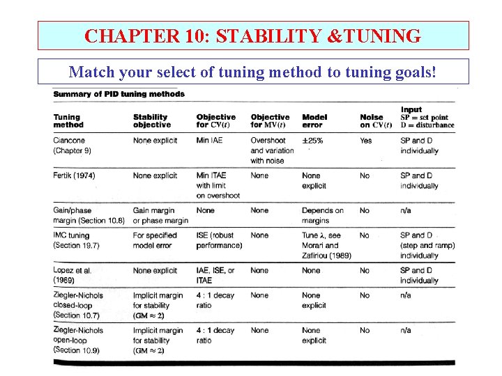
CHAPTER 10: STABILITY &TUNING Match your select of tuning method to tuning goals!

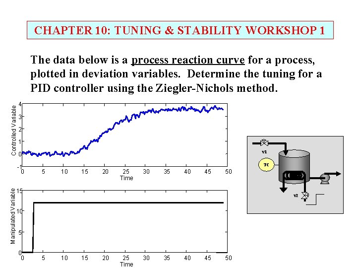
CHAPTER 10: TUNING & STABILITY WORKSHOP 1 Controlled Variable The data below is a process reaction curve for a process, plotted in deviation variables. Determine the tuning for a PID controller using the Ziegler-Nichols method. 4 3 2 1 0 v 1 -1 0 TC 5 10 15 20 25 Time 30 35 40 45 50 Manipulated Variable 15 v 2 10 5 0 0 5 10 15 20 25 Time 30 35 40 45 50

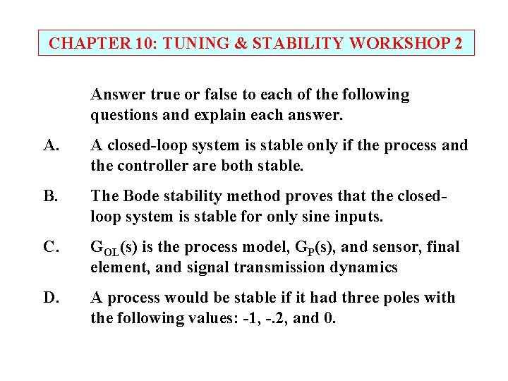
CHAPTER 10: TUNING & STABILITY WORKSHOP 2 Answer true or false to each of the following questions and explain each answer. A. A closed-loop system is stable only if the process and the controller are both stable. B. The Bode stability method proves that the closedloop system is stable for only sine inputs. C. GOL(s) is the process model, GP(s), and sensor, final element, and signal transmission dynamics D. A process would be stable if it had three poles with the following values: -1, -. 2, and 0.

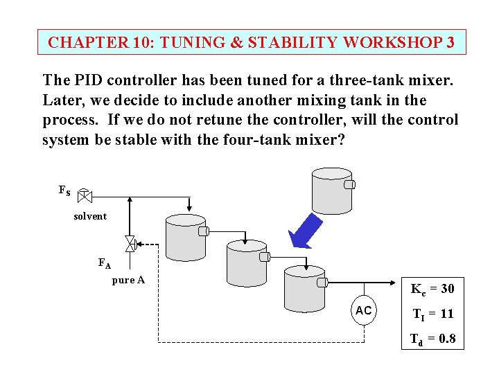
CHAPTER 10: TUNING & STABILITY WORKSHOP 3 The PID controller has been tuned for a three-tank mixer. Later, we decide to include another mixing tank in the process. If we do not retune the controller, will the control system be stable with the four-tank mixer? FS solvent FA pure A Kc = 30 AC TI = 11 Td = 0. 8

CHAPTER 10: STABILITY &TUNING When I complete this chapter, I want to be able to do the following. • Determine the stability of a process without control • Determine the stability of a closed-loop feedback control system • Use these approaches to learn how dead time affects stability. Lot’s of improvement, but we need some more study! • Read the textbook • Review the notes, especially learning goals and workshop • Try out the self-study suggestions • Naturally, we’ll have an assignment!

CHAPTER 10: LEARNING RESOURCES • SITE PC-EDUCATION WEB - Instrumentation Notes - Interactive Learning Module (Chapter 10) - Tutorials (Chapter 10) • S_LOOP - You can perform the stability and frequency response calculations uses menu-driven features. Then, you can simulate in the time domain to confirm your conclusions.

CHAPTER 10: SUGGESTIONS FOR SELF-STUDY 1. Determine the stability for the example in textbook Table 9. 2 (recommended tuning). Use the nominal process parameters. How much would KC have to be increased until the system became unstable? 2. Determine the Ziegler-Nichols tuning for the three-tank mixer process. Simulate the dynamic response using S_LOOP. 3. Discuss applying the Bode stability method to a process without control.

CHAPTER 10: SUGGESTIONS FOR SELF-STUDY 4. We do not want to operate a closed-loop system “too close” to the stability limit. Discuss measures of the closeness to the limit and how they could be used in calculating tuning constant values.