POWER SYSTEM COMMISSIONING AND MAINTENANCE PRACTICE DET 3103

POWER SYSTEM COMMISSIONING AND MAINTENANCE PRACTICE DET 310/3 CURRENT TRANSFORMER

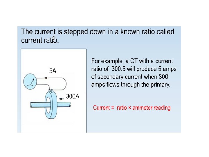
9. 0 INTRODUCTION Current or voltage instrument transformers are necessary for isolating the protection, control and measurement equipment from the high voltages of a power system It is a device used to measure large current by scaling large primary currents to smaller secondary current; for example from 1000 A to 1, 3 or 5 A. (1000/1, 1000/3, 1000/5)

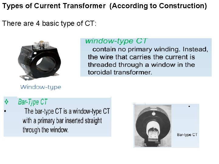
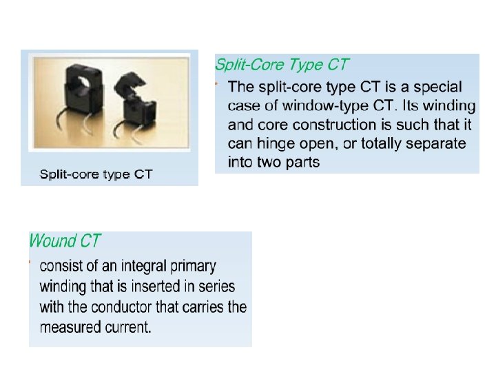
Types of Current Transformer (According to Construction) There are 4 basic type of CT:

Standards BS 3938 IEC 60044 -1 – Specifications of current Transformer, General requirements (formerly BS 3938) IEC 60044 -6 – Requirement for transient performance

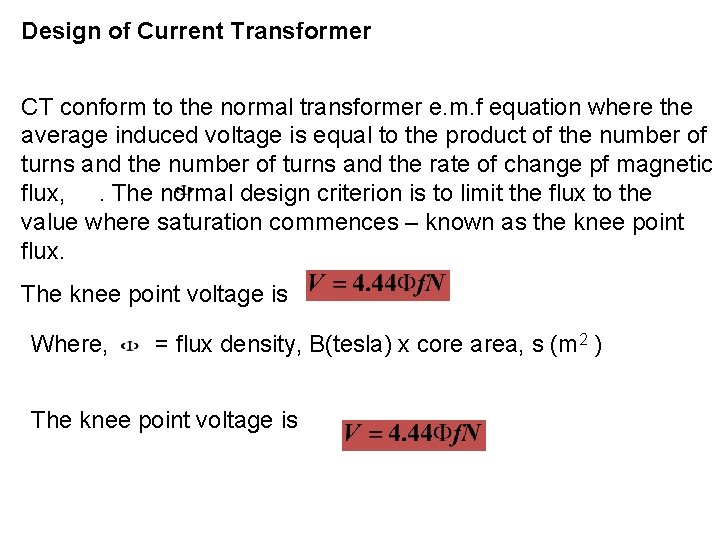
Design of Current Transformer CT conform to the normal transformer e. m. f equation where the average induced voltage is equal to the product of the number of turns and the rate of change pf magnetic flux, . The normal design criterion is to limit the flux to the value where saturation commences – known as the knee point flux. The knee point voltage is Where, = flux density, B(tesla) x core area, s (m 2 ) The knee point voltage is

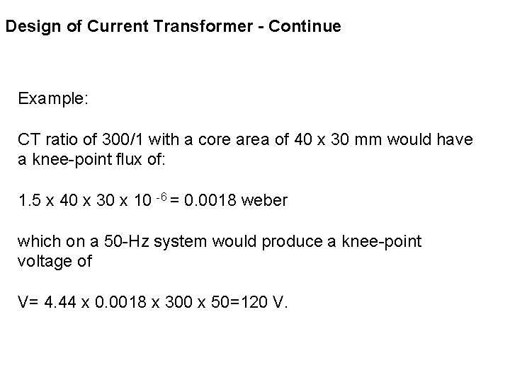
Design of Current Transformer - Continue Example: CT ratio of 300/1 with a core area of 40 x 30 mm would have a knee-point flux of: 1. 5 x 40 x 30 x 10 -6 = 0. 0018 weber which on a 50 -Hz system would produce a knee-point voltage of V= 4. 44 x 0. 0018 x 300 x 50=120 V.

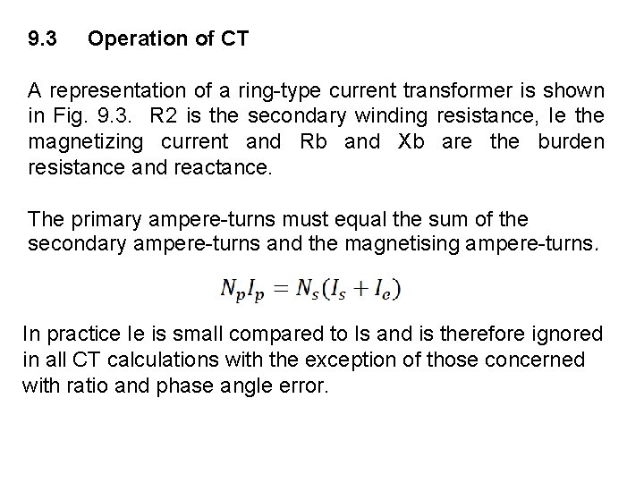
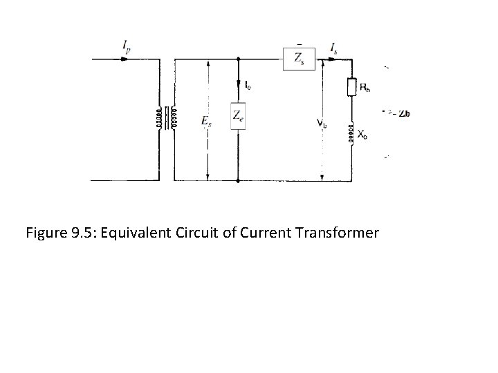
9. 3 Operation of CT A representation of a ring-type current transformer is shown in Fig. 9. 3. R 2 is the secondary winding resistance, Ie the magnetizing current and Rb and Xb are the burden resistance and reactance. The primary ampere-turns must equal the sum of the secondary ampere-turns and the magnetising ampere-turns. In practice Ie is small compared to Is and is therefore ignored in all CT calculations with the exception of those concerned with ratio and phase angle error.

Figure 9. 5: Equivalent Circuit of Current Transformer

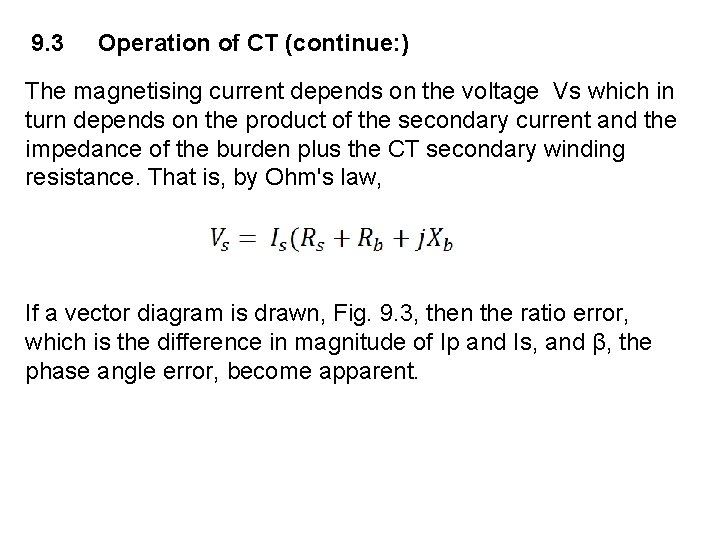
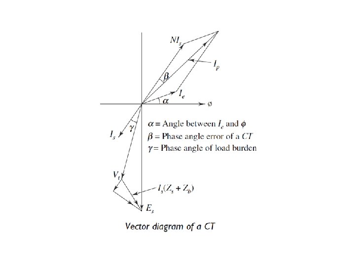
9. 3 Operation of CT (continue: ) The magnetising current depends on the voltage Vs which in turn depends on the product of the secondary current and the impedance of the burden plus the CT secondary winding resistance. That is, by Ohm's law, If a vector diagram is drawn, Fig. 9. 3, then the ratio error, which is the difference in magnitude of Ip and Is, and β, the phase angle error, become apparent.

9. 3 Operation of CT (continue: ) The magnetizing current Ie lags Vs by 90°. It can be seen if the burden is wholly resistive, then the ratio error would be a minimum.

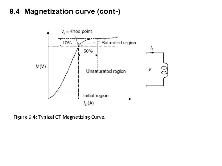
9. 4 Magnetization curve This curve is the best method of determining a CTs performance. It is a graph of the amount of magnetizing current required to generate an open-circuit voltage at the terminals of the unit. Due to the non-linearity of the core iron, it follows the B-H loop characteristic and comprises three regions, namely the initial region, unsaturated region and saturated region (Figure 9. 5)

9. 4 Magnetization curve (cont-) Figure 9. 4: Typical CT Magnetizing Curve.

9. 4 Magnetizing Curve (continue) The transition from the unsaturated to the saturated region of the open-circuit excitation characteristic is a rather gradual process in most core materials. This transition characteristic makes a CT not to produce equivalent primary current beyond certain point. This transition is defined by ‘kneepoint’ voltage in a CT, which decides its accurate working range. It is generally defined as the voltage at which a further 10% increase in volts at the secondary side of the CT requires more than 50% increase in excitation current. For most applications, it means that current transformers can be considered as approximately linear up to this point.

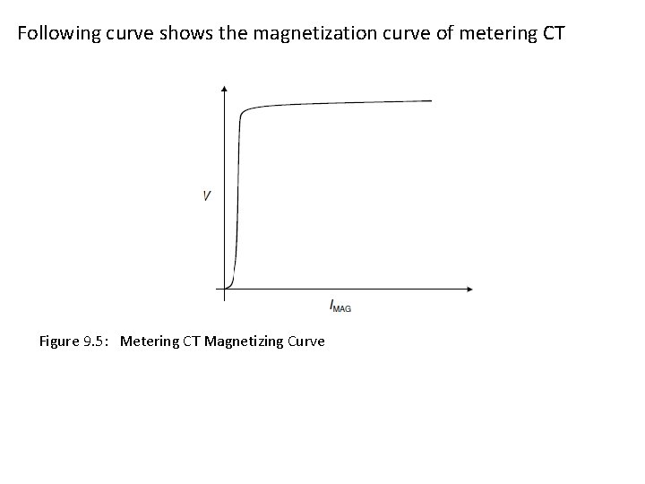
9. 7 Classification of CT - Measuring CT - Protection CT 9. 7. 1 Measurements Ct Instruments and meters are required to work accurately up to full -load current, but above this, it is advantageous to saturate and protect the instruments under fault conditions. Hence, it is common to have metering CTs with a very sharp knee-point voltage. A special nickel-alloy metal having a very low magnetizing current is used in order to achieve the accuracy.

9. 7. 1 Measurements Ct (cont-) Measurement CTs class are shown as: 0. 1 (Lab / calibration function) 0. 2 (Accurate revenue application) 0. 5 (Revenue application) 1. 0 (Normal application) 3. 0 (Non revenue application) 5. 0 (Estimate reading

Following curve shows the magnetization curve of metering CT Figure 9. 5: Metering CT Magnetizing Curve

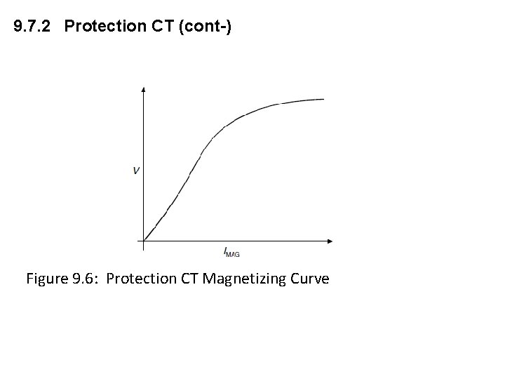
9. 7. 2 Protection CT Protective relays are not normally expected to give tripping instructions under normal conditions. On the other hand these are concerned with a wide range of currents from acceptable fault settings to maximum fault currents many times normal rating. Larger errors may be permitted and it is important that saturation is avoided wherever possible to ensure positive operation of the relays mainly when the currents are many times the normal current

9. 7. 2 Protection CT (cont-) Figure 9. 6: Protection CT Magnetizing Curve

9. 7. 2 Protection CT (cont-) Protection Class CT are as below: Protection class CTs are as below Class P ; Eg: 5 P 5, 5 P 10, 5 P 15, 5 P 20, 5 P 30 10 P 5, 10 P 10, 10 P 15, 10 P 20, 10 P 30 Class PX; Eg 0. 1 PX 100 R 5, 0. 05 PX 1500 R 12

9. 8 CTs Specification A current transformer is normally specified in terms of: • A rated burden at rated current • An accuracy class • Rated Primary/Secondary Current • Knee Point Voltage- Class PS and PX • Instrument Security factor

9. 8. 1 Rated Primary and Secondary Current This is the value of the primary and secondary current which is marked on the rating plate of the current transformer and on which the performance of the CT is specified by the manufacturer. Eg: 1000/1 15 VA 10 P 10 Primary current : 1000 A; Secondary current : 1 A

9. 8. 1 CTs Burden The burden of a current transformer is indicated in its nameplate. The burden is rated in VA. such as 15 VA or 25 VA. The rated VA indicates the load the transformer can take. The current transformer is connected to a measuring instrument or a protective relay by means of wires. The burden on the current transformer is imposed by the connected device and the impedance of the connecting wires which connect it. The VA load of the device can be obtained from the datasheet provided by the manufacturer. The total burden is the sum of the burden of the connected devices and the resistance of the wires. The inductive component of the wire impedance is usually neglected as it is minimal.

9. 8. 1 CTs Burden The burden of a current transformer can increase over time as the resistance of the connecting wires may slightly increase due to age, change in temperature and loosening of connections. Hence, the current transformer should never be loaded to 100% of its capacity. For Class PX, however, the rated burden is in ohm. Eg: For Class P CT: 1000/1 15 VA 10 P 5 – rated burden is 15 VA For Class PX 0. 05 PX 1500 R 12 - rated burden is 12 ohm

9. 8. 1 CTs Burden (cont-) All burdens are connected in series and the increase in impedance increases the burden on the current transformer. A current transformer is unloaded if the secondary winding is shortcircuited as under this condition the VA burden is zero because the voltage is zero. The errors of transformation depend on the angle of the burden as well as its impedance

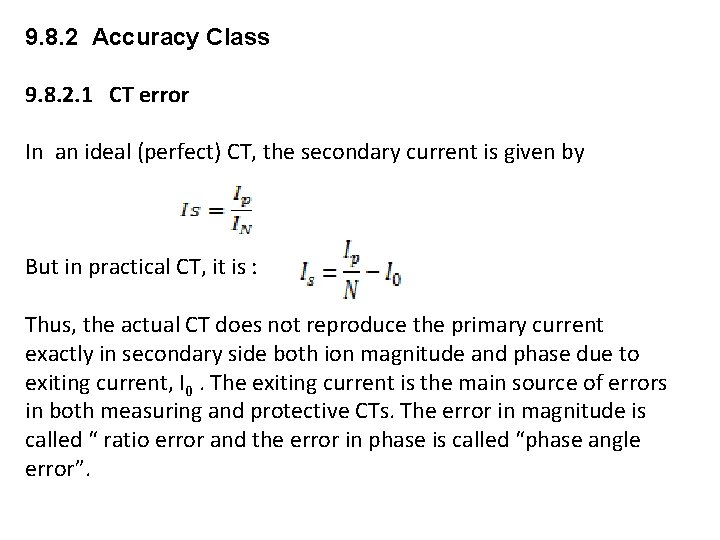
9. 8. 2 Accuracy Class 9. 8. 2. 1 CT error In an ideal (perfect) CT, the secondary current is given by But in practical CT, it is : Thus, the actual CT does not reproduce the primary current exactly in secondary side both ion magnitude and phase due to exiting current, I 0. The exiting current is the main source of errors in both measuring and protective CTs. The error in magnitude is called “ ratio error and the error in phase is called “phase angle error”.

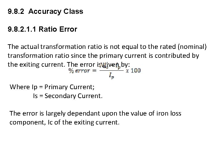
9. 8. 2 Accuracy Class 9. 8. 2. 1. 1 Ratio Error The actual transformation ratio is not equal to the rated (nominal) transformation ratio since the primary current is contributed by the exiting current. The error is given by: Where Ip = Primary Current; Is = Secondary Current. The error is largely dependant upon the value of iron loss component, Ic of the exiting current.

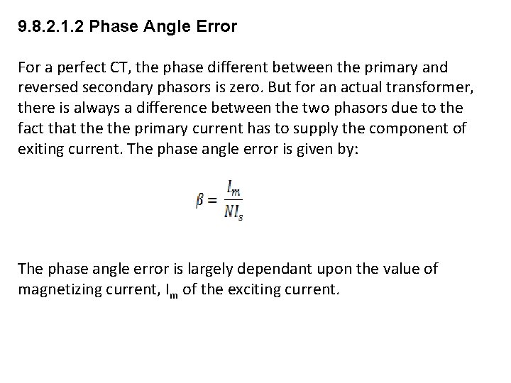
9. 8. 2. 1. 2 Phase Angle Error For a perfect CT, the phase different between the primary and reversed secondary phasors is zero. But for an actual transformer, there is always a difference between the two phasors due to the fact that the primary current has to supply the component of exiting current. The phase angle error is given by: The phase angle error is largely dependant upon the value of magnetizing current, Im of the exciting current.

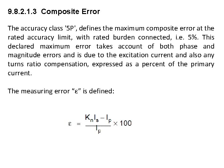
9. 8. 2. 1. 3 Composite Error The accuracy class '5 P', defines the maximum composite error at the rated accuracy limit, with rated burden connected, i. e. 5%. This declared maximum error takes account of both phase and magnitude errors and is due to the excitation current and also any turns ratio compensation, expressed as a percent of the primary current. The measuring error “ε” is defined:

9. 8. 2 Accuracy Class Standard quoted for accuracy class For measuring CT: Measuring transformers are classified into 0. 1, 0. 3, 0. 5, 1. The values indicate the percentage error at the rated primary current. Thus a 100/5 transformer with 0. 3 accuracy will have a maximum error of 0. 3 when a current of 100 A passes through the primary.

9. 8. 2 Accuracy Class and Accuracy Limit Factor (cont-) For Protection CT 5 P 10 P The accuracy class '5 P', defines the maximum composite error at the rated accuracy limit, with rated burden connected, i. e. 5%. This declared maximum error takes account of both phase and magnitude errors and is due to the excitation current and also any turns ratio compensation, expressed as a percent of the primary current. Standard ALF are: 5, 10, 15, 20 and 30

9. 8. 2 Accuracy Class and Accuracy Limit Factor

9. 8. 2 Accuracy Class and Accuracy Limit Factor (cont-)

9. 8. 2 Accuracy Class and Accuracy Limit Factor (cont-) Table – limits of current, phase displacement and composite error for protection CT

9. 8. 2 Accuracy Class and Accuracy Limit Factor (cont-) Standard ALF are: 5, 10, 15, 20 and 30 For Example, 5 VA, 5 P 10 CT will transform primary current of up to 10 x its rating and remain within the composite accuracy limit of 5% with a burden of 5 VA (at rated current) connected to the CT secondary.

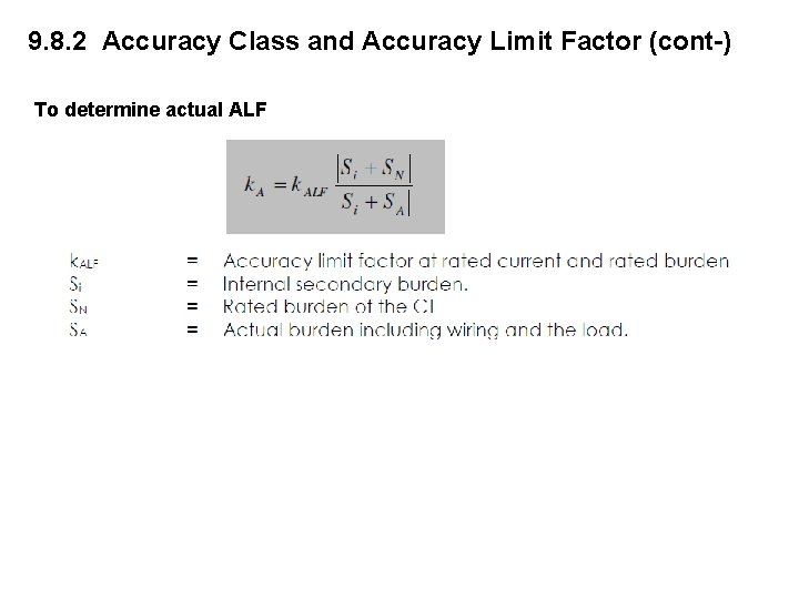
9. 8. 2 Accuracy Class and Accuracy Limit Factor (cont-) To determine actual ALF

9. 8. 2 Accuracy Class and Accuracy Limit Factor (cont-) Example: The internal secondary coil resistance of a CT is 0. 07 ohm and secondary burden (R relay + R wire) is 0. 117 ohm. CT details are 300/5, 5 P 20, 10 VA. Determine actual ALF: Solutions:

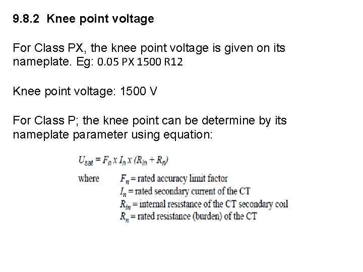
9. 8. 2 Knee point voltage For Class PX, the knee point voltage is given on its nameplate. Eg: 0. 05 PX 1500 R 12 Knee point voltage: 1500 V For Class P; the knee point can be determine by its nameplate parameter using equation:

9. 8. 2 Knee point voltage (continue) Example: Find Knee point voltage for a CT with following parameters: 1000/5 ; 20 VA, 10 P 20 ; R int = 0. 07 ohm; Solutions:

9. 8. 2 Instrument Security Factor This is the ratio of instrument limit primary current to the rated primary current. A high SF will mean a high transformation of the primary current and can damage instrument connected to its secondary. For measuring instruments, it is kept low as it is required to measure only the normal current and not the fault current.

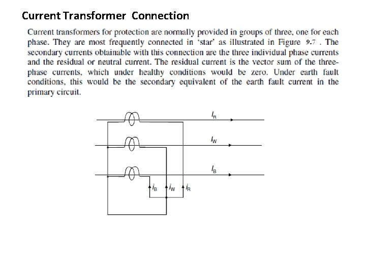
Current Transformer Connection

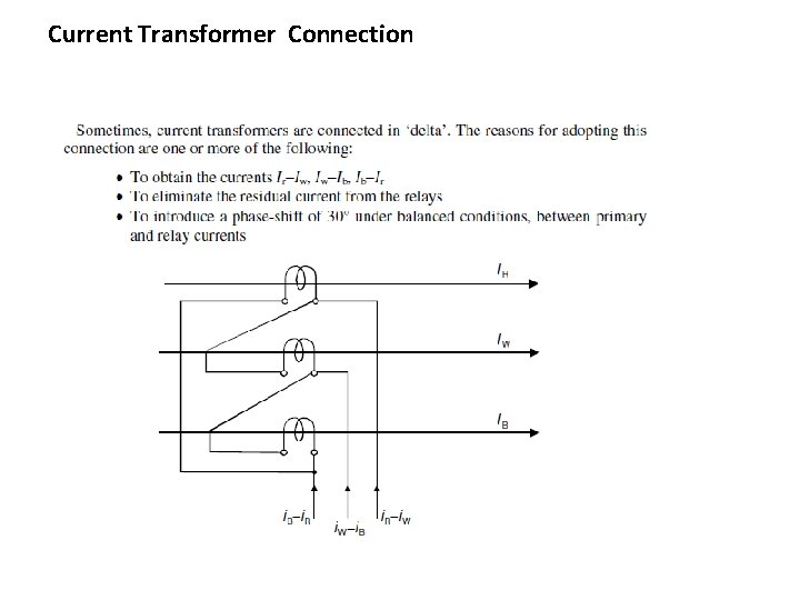
Current Transformer Connection

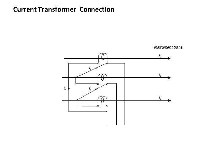
Current Transformer Connection

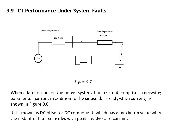
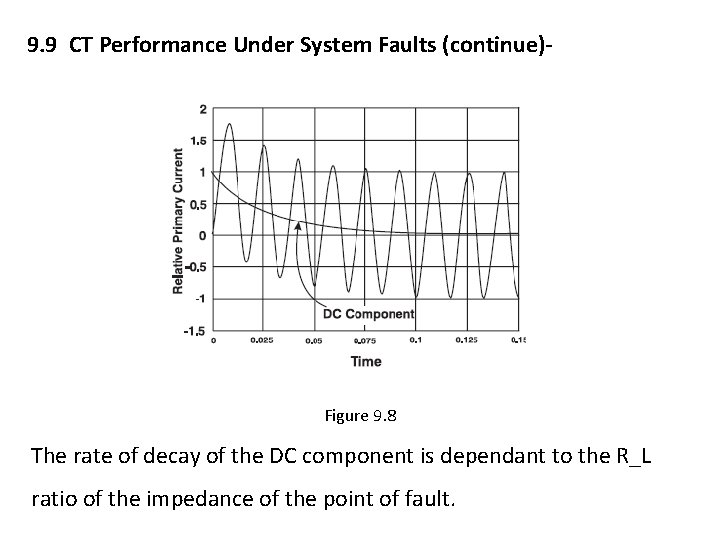
9. 9 CT Performance Under System Faults Figure 9. 7 When a fault occurs on the power system, fault current comprises a decaying exponential current in addition to the sinusoidal steady-state current, as shown in Figure 9. 8 Its is known as DC offset or DC component, which has a maximum value when the instant of fault coincides with peak steady-state current.

9. 9 CT Performance Under System Faults (continue)- Figure 9. 8 The rate of decay of the DC component is dependant to the R_L ratio of the impedance of the point of fault.

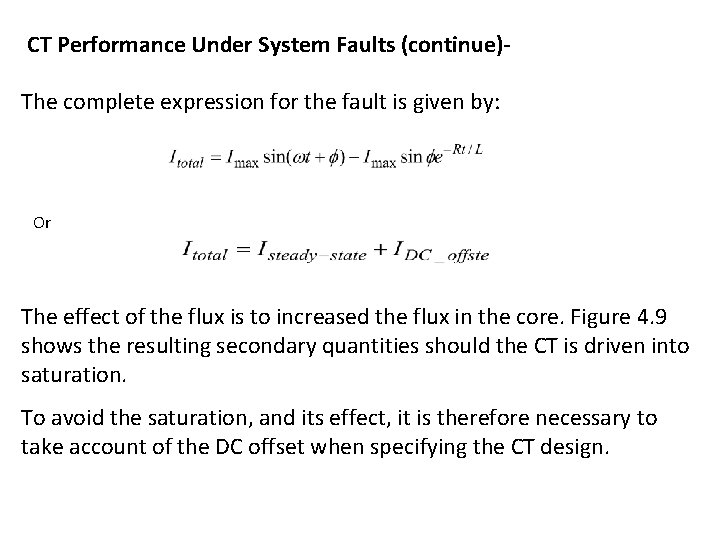
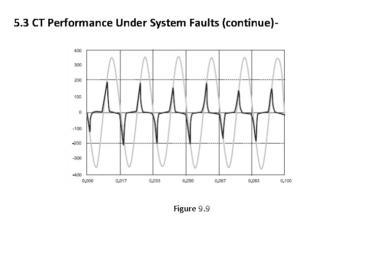
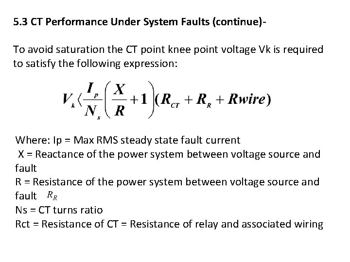
CT Performance Under System Faults (continue)The complete expression for the fault is given by: Or The effect of the flux is to increased the flux in the core. Figure 4. 9 shows the resulting secondary quantities should the CT is driven into saturation. To avoid the saturation, and its effect, it is therefore necessary to take account of the DC offset when specifying the CT design.

5. 3 CT Performance Under System Faults (continue)- Figure 9. 9

5. 3 CT Performance Under System Faults (continue)To avoid saturation the CT point knee point voltage Vk is required to satisfy the following expression: Where: Ip = Max RMS steady state fault current X = Reactance of the power system between voltage source and fault R = Resistance of the power system between voltage source and fault Ns = CT turns ratio Rct = Resistance of CT = Resistance of relay and associated wiring

5. 4 TESTING AND COMMISIONING OF CT Physical check/inspection: i. Inspect physical conditions: no damage, no missing hardware and correct vertical and horizontal alignment ii. Correct oil level/check for oil leak (if applicable); iii. Verify correct mounting of the CT, earth connections and electrodes iv. Check cable entrance for tidiness, protection from sharp metallic edges, no injury in insulation and vermin proof. v. Visual check of primary and secondary circuits against approved drawings. vi. Using circuit diagram, check that P 1 and P 2 primary terminals are correctly connected.

5. 4 TESTING AND COMMISIONING OF CT Electrical Test The basic commissioning tests usually carried out on CTs consists of Ø Check on CT position Ø Flick Test Ø magnetizing curves Ø Burden Ø Insulation resistance test Ø primary injections Ø on load test

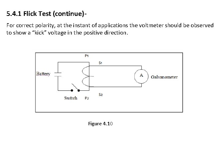
5. 4. 1 Flick Test Objectives: to prove that a CT has been manufactured and installed with the correct polarity. If the current flows into the primary in a certain direction w. r. t to voltage, the secondary curent must flow out of the secondary winding in a corresponding and prescribe direction. For the flick test, DC voltage of 9 Volts should be connected with its postitive pole to terminal P 1 and negative terminal to P 2. To verify the polarity, a galvanometer selected to measures DC quantities should be connected with its positive pole to terminal S 1 and negative pole to terminal S 2.

5. 4. 1 Flick Test (continue)For correct polarity, at the instant of applications the voltmeter should be observed to show a “kick” voltage in the positive direction. Figure 4. 10

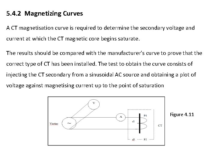
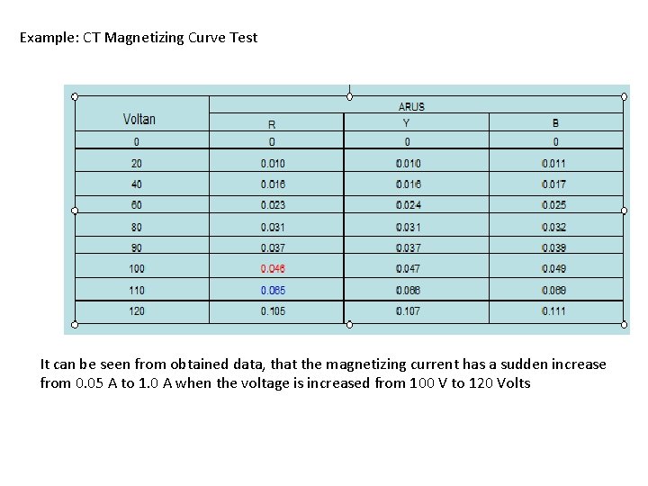
5. 4. 2 Magnetizing Curves A CT magnetisation curve is required to determine the secondary voltage and current at which the CT magnetic core begins saturate. The results should be compared with the manufacturer’s curve to prove that the correct type of CT has been installed. The test to obtain the curve consists of injecting the CT secondary from a sinusoidal AC source and obtaining a plot of voltage against magnetising current up to the point of saturation Figure 4. 11

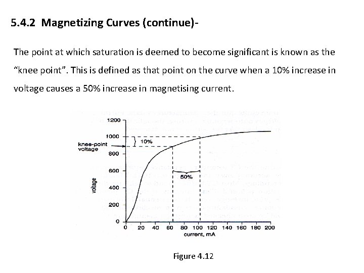
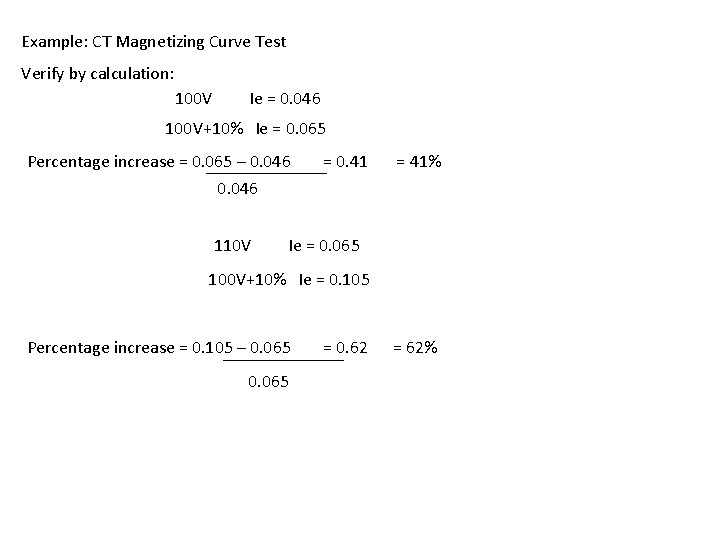
5. 4. 2 Magnetizing Curves (continue)The point at which saturation is deemed to become significant is known as the “knee point”. This is defined as that point on the curve when a 10% increase in voltage causes a 50% increase in magnetising current. Figure 4. 12

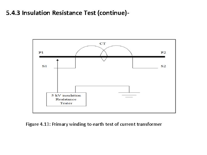
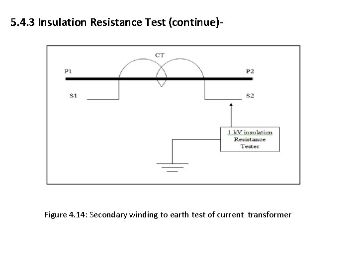
5. 4. 3 Insulation Resistance Test The objective insulation resistance test current transformer (CT) is to ensure the CT windings have good insulation to ground. For testing, we use the 1 k. V, 5 k. V insulation tester. Use 1 k. V insulation tester to check the insulation between secondary winding and earth. Use 5 k. V insulation testers to check the insulation between the primary windings and earth and between primary and secondary winding and earth

5. 4. 3 Insulation Resistance Test (continue)- Figure 4. 13: Primary winding to earth test of current transformer

5. 4. 3 Insulation Resistance Test (continue)- Figure 4. 14: Secondary winding to earth test of current transformer

Example: CT Magnetizing Curve Test It can be seen from obtained data, that the magnetizing current has a sudden increase from 0. 05 A to 1. 0 A when the voltage is increased from 100 V to 120 Volts

Example: CT Magnetizing Curve Test Verify by calculation: 100 V Ie = 0. 046 100 V+10% Ie = 0. 065 Percentage increase = 0. 065 – 0. 046 = 0. 41 = 41% 0. 046 110 V Ie = 0. 065 100 V+10% Ie = 0. 105 Percentage increase = 0. 105 – 0. 065 = 0. 62 = 62%

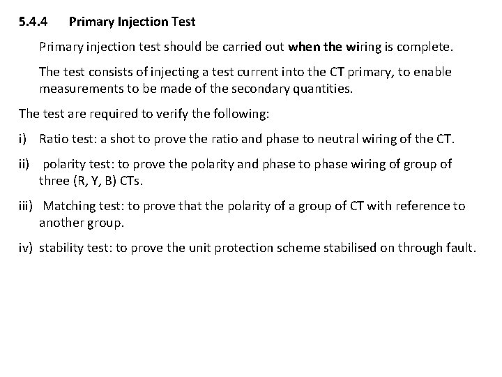
5. 4. 4 Primary Injection Test Primary injection test should be carried out when the wiring is complete. The test consists of injecting a test current into the CT primary, to enable measurements to be made of the secondary quantities. The test are required to verify the following: i) Ratio test: a shot to prove the ratio and phase to neutral wiring of the CT. ii) polarity test: to prove the polarity and phase to phase wiring of group of three (R, Y, B) CTs. iii) Matching test: to prove that the polarity of a group of CT with reference to another group. iv) stability test: to prove the unit protection scheme stabilised on through fault.

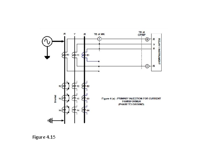
Figure 4. 15

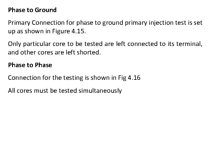
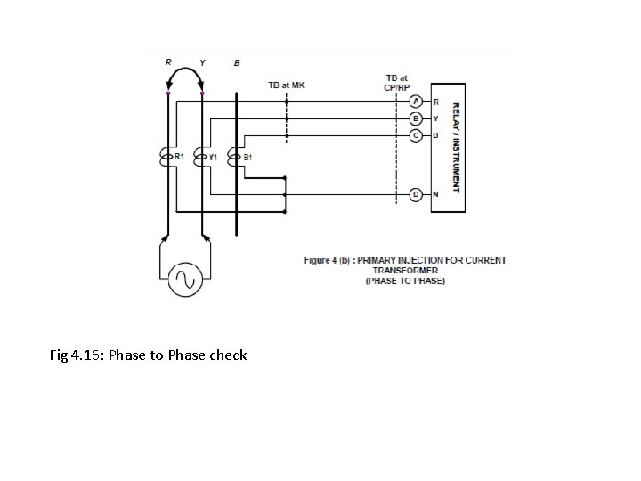
Phase to Ground Primary Connection for phase to ground primary injection test is set up as shown in Figure 4. 15. Only particular core to be tested are left connected to its terminal, and other cores are left shorted. Phase to Phase Connection for the testing is shown in Fig 4. 16 All cores must be tested simultaneously

Fig 4. 16: Phase to Phase check