POISSON REGRESSION 1 Models for counts The Poisson

POISSON REGRESSION

1. Models for counts: • The Poisson probability density function is given by • The mean and variance of the Poisson distribution is • Poisson regression models allow researchers to examine the relationship between predictors and count outcome variables.

Examples • The Poisson distribution arises in many biological and medical contexts where counts are involved: – The number of bacterial colonies in a dish – The number of trees in an area of land – The number of children an individual has – The number of nucleotide base substitutions in a gene over a period of time – The number of deaths in a group of patients over a study period

The model for counts • ln( i) = 0 + 1 xi 1 + 2 xi 2 + …+ pxip , Ø We need the logarithm, since 0 + 1 xi 1 + 2 xi 2 + …+ pxip can take any real value, but we are modelling counts ( i), so we want it to be >0.

Example • Respiratory deaths were counted in Athens between 1988 and 1991 • We have 4 variables: – Cases: the number of deaths – Pop: the population of each age group – Age: the categorical age group; one of 40 − 54, 55 − 59, 60 − 64, 65 − 74 or > 74 • Questions of interest: How does the expected number of deaths vary by age? • ln( i) = 0 + 1 I 40− 54 + 2 I 55 -59 + 3 I 60 -64 + 4 I 65 -74

What about modelling rates? • If all patients are assumed to be followed-up for the same time interval, a rate is unnecessary • But if there is variation in the time each individual is followed-up, modelling the count of deaths would be misleading.

2. Models for rates Example The British doctors study: The classical cohort study by Doll et al which was used (among other objectives) to investigate the effect of smoking on coronary heart disease (CHD) among male British doctors. agegrp smoke deaths Pyrs 1 1 32 52407 2 1 104 43248 3 1 206 28612 4 1 186 12663 5 1 102 5317 1 0 2 18790 2 0 12 10673 3 0 28 5710 4 0 28 2585 5 0 31 1462 With age groups being 1: 35 -44, 2: 45 -54, 3: 55 -64, 4: 65 -74, 5: 75+ The crude CHD death rate for the non-smokers is 101/39220 = 0. 0026 and for the smokers 630/142247 = 0. 0044. Therefore the ratio of non smokers compared to smokers is 0. 6, i. e. , non-smokers have a reduced rate of CHD deaths.

Models for rates • Imagine events which occur independently in time intervals ti with rates i , • Yi random variables denoting the numbers of events in the corresponding ti and they have Poisson distributions with means i= i ti – Poisson models handle exposure variables by using simple algebra to change the dependent variable from a rate into a count.

Models for rates • If the rate is count/exposure, multiplying both sides of the equation by exposure moves it to the right side of the equation. • • • The Poisson model is a regression model of the mean i on p explanatory variables xi 1, xi 2, …, xip , where the link function is the log function. The model we are interested in is a model for the rates i , i. e. , ln( i) = 0 + 1 xi 1 + 2 xi 2 + …+ pxip , and because i= i ti. ln( i) – ln(ti ) = 0 + 1 xi 1 + 2 xi 2 + …+ pxip , thus ln( i) = ln(ti ) + 0 + 1 xi 1 + 2 xi 2 + …+ pxip , The Poisson model includes the offset term –ln(ti)- representing the logperson years which has a coefficient equal to one. • Using the offset is just a way of accounting for population sizes, which could vary by time. • The coefficients 1 … p represent the effect of each of the xi 1, xi 2 , …, xip on the log of rates i

3. Assumptions for Poisson regression: • The distribution of deaths in each time interval will be well approximated by a Poisson distribution if the following is true – Only one event can occur in each interval – Low event rates: The proportion of patients who have the event/disease of interest in each risk group should be small. – The rate parameter λ is the same across all intervals – The time intervals are independent, i. e the probability of observing an event in an interval l does not depend on whether we observed event(s) in any other interval • Of note, the denominators of rates used in Poisson regressions is often patient-years rather than patients. • In fact, it depends on what rate we want to estimate (see examples below)

Poisson versus Survival analysis models • Poisson regression is a very useful tool when we need to estimate rates i. e. for analyzing cohort studies • If we have detailed individual-level data (accurate data on the follow-up time for each of the cohort participants) , we can apply the more sophisticated approaches that have been developed in the field of survival analysis

4. Examples: Define Si = 1 xi 1 where xi 1 is an indicator with 1 denoting that group i consists of smokers and 0 otherwise. Define Ai = 2 xi 2 + 3 xi 3 + 4 xi 4 + 5 xi 5 , where xij , j=2, …, 5 are indicators with 1 if group i is the age class j and 0 otherwise. Now j represent the effect of the age groups on the log rate of CHD deaths. What we want to investigate are: the effect of smoking on CHD rate, and the effect of smoking on CHD rate, having adjusted for age.

Model 1: smoking ln(μi) = ln (ti) + β 0 + Si Fitting this model through Stata we have the following: xi : poisson deaths i. smokes, e (pyrs) i. smokes Ismoke_0 -1 (naturally coded; Ismoke_0 omitted) Iteration 0: log likelihood = -480. 77391 Iteration 1: log likelihood = -480. 52234 Iteration 2: log likelihood = -480 52206 Iteration 3: log likelihood = -480. 52206 Poisson regression Number of obs LR chi 2(1) Prob > chi 2 Log likelihood = -480. 52206 Pseudo R 2 deaths Coef. Std. Err. Ismoke_1 . 5422211 . 1071834 _cons -5. 961822. 0995037 pyrs (exposure) z = 10 = 29. 09 = 0. 0000 = 0. 0294 P [95% Conf Interval] 5. 059 <0. 001 . 3321454 . 7522968 -59. 916 <0. 001 -6. 156845 -5. 766798 The interpretation of the parameter estimates is as follows. : the estimated log rate for non-smokers. : the estimated difference in log rates between non-smokers and smokers. : the estimated crude ratio between non-smokers and smokers.

Model 2: adjusting for age ln(μi) = ln (ti) + Si + Ai Fitting this model through Stata we have the following: xi : poisson deaths i. smokes i. agegrp, e (pyrs) deaths Ismoke_1 Iagegr _ 2 Iagegr_ 3 Iagegr_ 4 Iagegr_ 5 _cons pyrs Coef. . 3545356 1. 484007 2. 627505 3. 350493 3. 700096 -7. 919326 (exposure) Std. Err. . 1073741. 1951034. 1837273. 1847992. 1922195. 1917618 z 3. 302 7. 606 14. 301 18. 130 19. 249 -41. 298 P> 0. 001 0. 000 [95% Conf. 1440862 1. 101611 2. 267406 2. 988293 3. 323353 -8. 295172 Interval]. 564985 1. 866403 2. 987604 3. 712693 4. 07684 -7. 543479 The age-adjusted rate ratio, comparing smokers with non-smokers, is: e 0. 3545 = 1. 43 (similar to M-H=1. 39), with 95% CI (e 0. 3545 -1. 96 X 0. 1074 , e 0. 3545+1. 96 X 0. 1074 ) = (1. 16, 1. 76). Assumes effects of smoke and age combine multiplicatively (i. e. there is no significant interaction between them)

5. Testing hypotheses in Poisson regression 1. Wald test (given directly in STATA output) 2. the likelihood ratio test. Testing for effect modification Poisson model in its simple form assumes no interaction between explanatory variables But we can check whether the effect of the exposure (e. g. smoke) differs according to the levels of the potential confounder (e. g. age) Using the LR test and the nested models

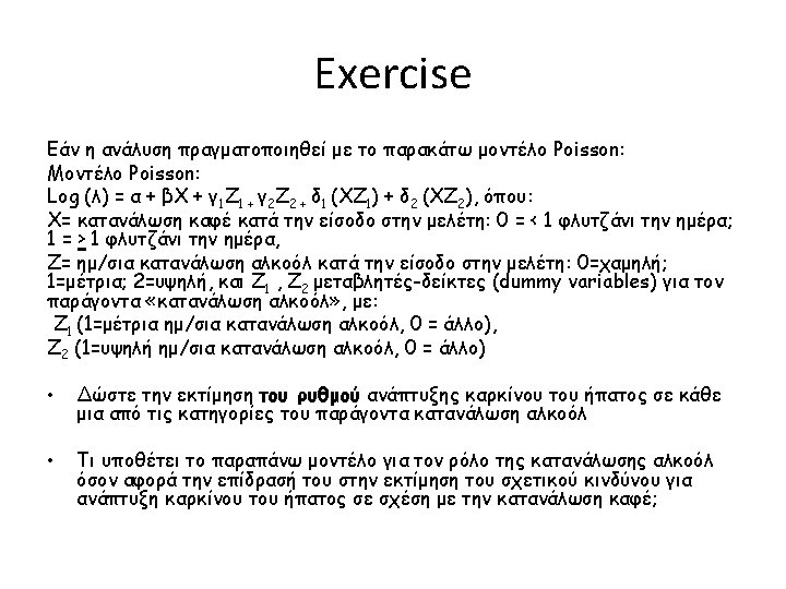
The model in full Stratum (Z=0, 1, 2) 0 1 2 0 a a + γ 1 a + γ 2 Log rates of outcome The model in full In multiplicative form Exposure (X) 1 a+β a + γ 1 + β a + γ 2 + β Stratum (Z=0, 1, 2) 0 1 2 0 λc λ c φ1 λc φ2 Exposure (X) 1 λc θ φ 2 rates of outcome Log (λ) = α + βx + γ 1 z 1 + γ 2 z 2 What is the difference in the log rates in stratum 0 between exposed and unexposed? In stratum 1? What do we assume here?

Interactions (effect modification) Log (λ) = α + βx + γ 1 z 1 + γ 2 z 2 + δ 1 (xz 1) + δ 2 (xz 2) Stratum 0 1 2 0 a a + γ 1 a + γ 2 Exposure 1 a + β a + γ 1 + β + δ 1 a + γ 2 + β + δ 2 What is the difference in the log rates in stratum 0 between exposed and unexposed? In stratum 1? What do we assume here? In multiplicative form Stratum 0 1 2 0 λc λc φ 1 λc φ 2 Exposure 1 λc θ φ 1 ρ 1 λc θ φ 2 ρ 2

Poisson regression - Stratification Remember the Whitehall Study with grade of work (exposure) and age (confounder) xi : poisson deaths i. grade*agegrp, e (pyrs) irr Deaths RR SE z p-value 95% CI Test for interaction xi : poisson deaths i. grade i. agegrp, e (pyrs) est store B lrtest A B likelihood-ratio test chi 2(5) = 10. 43, (Assumption: B nested in A) Prob > chi 2 = 0. 0640

Quantitative exposure in Poisson regression • If explanatory variable is quantitative (or ordered) can use Poisson model to test for linearity. • Stronger assumption than treating as categorical since uses fewer parameters - assumes log rate changes linearly across explanatory variable. • Caution: this is strong assumption since very few relationships are exactly log-linear • Only one parameter in model - change in log rate per unit of variable. • e. g. log λ = b 0 + Age

Quantitative exposure in Poisson regression (cont. ) • LRT compares: – Model 1: age categorical -no assumption of how log rate changes – Model 2: age quantitative - assumes log rate changes linearly • H 0: association is log-linear vs. • H 1: association is not log-linear

Quantitative exposure in Poisson regression (cont. ) • If exposure is quantitative, interpretation is “change in log rate per unit change”. • Imagine age as the exposure – how is it coded? – If age categorical is coded as groups of years, e. g, in 5 years groups as 1, 2, 3, 4, …then jump of one unit represents 5 -year jump – if values of the categories were 40, 45, 50, 55, …, then jump of one unit represents 1 -year jump

Quantitative exposure in Poisson regression (cont. ) • In STATA: e. g age coded: 40, 55, 60, 65, 70, 75, 80 (agegrp) xi : poisson deaths i. grade agegrp, e (pyrs) Deaths rate SE z p 95% CI -------+-------------------------------------------Igrade_2 | 1. 394941. 2350773 1. 975 0. 048 1. 00256 1. 940892 Agegrp | 1. 089857. 0112403 8. 343 0. 000 1. 068048 1. 112112 --------------------------------------------------1 unit jump = 1 year in age RR increases by 1. 089 for each 1 -year increase in age Approx. 1. 0895 = 1. 53 over 5 years

Quantitative exposure in Poisson regression (cont. ) • If same groups of age were grouped as 1, 2, 3, 4…(agegrp) xi : poisson deaths i. grade agegrp, e (pyrs) Deaths log(rate) SE z p 95% CI ------+----------------------------------------_Igrade_2 | 1. 396122. 2355799 1. 98 0. 048 1. 002981 1. 943364 Agegrp | 1. 552698. 0809653 8. 44 0. 000 1. 401848 1. 719779 --------------------------------------------------1 unit jump = 5 years in age RR increases by 1. 553 for each 5 -year increase in age

6. More on the offset • As we mentioned, Poisson regression may also be appropriate for rate data, – the rate is a count of events divided by some measure of that unit's exposure (a particular unit of observation). • Examples: – biologists may count the number of tree species in a forest: events would be tree observations, exposure would be unit area, and rate would be the number of species per unit area. – Demographers may model death rates in geographic areas as the count of deaths divided by person−years. – Event rates can be calculated as events per unit time, which allows the observation window to vary for each unit.

More on the offset • In these examples, exposure is: – unit area – person−years – unit time • This is handled as an offset, where the exposure variable enters on the right-hand side of the equation, but with a parameter estimate (for log(exposure)) constrained to 1. Ø Using the offset is a way of accounting for population sizes, which could vary not only by time but with age, region, area etc.

More on the offset • The fact that an offset variable is required to have a coefficient of 1 allows it to be part of the rate. • It allows you to theoretically move it back to the right side of the equation to turn your rate back into a count. • by defining an offset variable, we are only adjusting for the amount of opportunity an event has.

More on the offset Let’s assume individuals in a rehab center. Including time in the offset, means that we assume that every day in rehab makes a patient equally likely to have an aggressive incident. Each day is simply an opportunity for an incident. A patient in for 20 days is twice as likely to have an incident as a patient in for 10 days. Ø We assume that the likelihood of events is not changing over time (λ is constant for all time intervals). • If, for example, it takes patients a few weeks to learn the consequences of aggressive behavior, then stop or lessen their rates, then time is not just a matter of exposure. • Likewise, if patients start becoming more agitated after being in a program after a few months, so that the longer residence time is actually creating more aggression, then time is not just a matter of exposure. • In either of these cases, number of days in a program would serve better as a predictor than as an exposure variable. As a predictor, the coefficient will be estimated from the data, not set to 1. •

More on the offset Let’s assume children in the first grade. Including time in the offset, means that we assume that every day in school makes a child equally likely to learn one new word. Each day is simply an opportunity for new word to be learned. A child in the first 20 days is twice as likely to learn a new word as a child in the first 10 days. Ø We assume that the likelihood of learning new words is not changing over time (λ is constant for all time intervals). • If, for example, it takes children a few weeks to get used to the new environment, then the number of words learned increases, then time is not just a matter of exposure. • Similarly, if children start learning other things (e. g. phrases), so that the number of words learned decreases, then time is not just a matter of exposure. • In either of these cases, time in school would serve better as a predictor than as an exposure variable. As a predictor, the coefficient will be estimated from the data, not set to 1. •

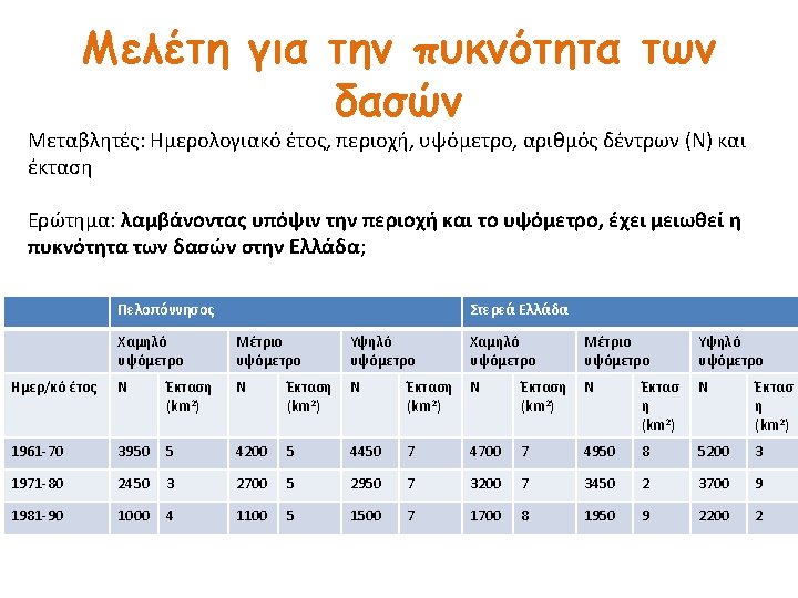
Example 1. 2. 3. 4. 5. 6. 7. 8. 9. 10. 11. 12. 13. 14. 15. 16. 17. 18. +---------------------------+ | cyear region altitude N Surface | |---------------------------| | 1960 -1970 Peloponisos low 3950 5 | | 1960 -1970 Peloponisos moderate 4200 5 | | 1960 -1970 Peloponisos high 4450 7 | | 1960 -1970 Sterea low 4700 7 | | 1960 -1970 Sterea moderate 4950 8 | | 1960 -1970 Sterea high 5200 3 | |---------------------------| | 1971 -1980 Peloponisos low 2450 3 | | 1971 -1980 Peloponisos moderate 2700 5 | | 1971 -1980 Peloponisos high 2950 7 | | 1971 -1980 Sterea low 3200 5 | | 1971 -1980 Sterea moderate 3450 2 | | 1971 -1980 Sterea high 3700 9 | |---------------------------| | 1981 -1990 Peloponisos low 1000 4 | | 1981 -1990 Peloponisos moderate 1100 5 | | 1981 -1990 Peloponisos high 1500 7 | | 1981 -1990 Sterea low 1700 8 | | 1981 -1990 Sterea moderate 1950 9 | | 1981 -1990 Sterea high 2200 2 | +---------------------------+

Example- The model. poisson N i. cyear i. region i. altitude, e(Surface) Poisson regression Log likelihood = -5113. 6953 Number of obs LR chi 2(5) Prob > chi 2 Pseudo R 2 = = 18 9766. 87 0. 0000 0. 4885 ---------------------------------------N | Coef. Std. Err. z P>|z| [95% Conf. Interval] -------+--------------------------------cyear | 1971 -1980 | -. 2859798. 0098027 -29. 17 0. 000 -. 3051928 -. 2667668 1981 -1990 | -1. 070379. 011933 -89. 70 0. 000 -1. 093767 -1. 04699 | region | Sterea |. 1747286. 0086865 20. 11 0. 000. 1577034. 1917539 | altitude | moderate |. 0460915. 0106708 4. 32 0. 000. 0251771. 067006 high |. 0698382. 0107716 6. 48 0. 000. 0487262. 0909501 | _cons | 6. 53408. 0102482 637. 58 0. 000 6. 513994 6. 554166 ln(Surface) | 1 (exposure) ---------------------------------------

Example- Interpretation • (e 0. 17 -1)*100=19. 1% • 19. 1% more trees per square km in Sterea compared to Peloponisos • (1 -e-0. 28)*100=24. 9% less trees per square km in 1971 -80 compared to 1960 -70 • (1 -e-1. 07)*100=65. 7% less trees per square km in 1981 -90 compared to 1960 -70

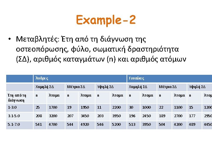
The dataset 1. 2. 3. 4. 5. 6. 7. 8. 9. 10. 11. 12. 13. 14. 15. 16. 17. 18. +------------------------------+ | group time gender pactiv~y rate N fractu~s | |------------------------------| | 1 1 -3. 0 Woman low. 03 1000 30 | | 2 1 -3. 0 Woman moderate. 02 1100 22 | | 3 1 -3. 0 Woman high. 01 1500 15 | | 4 1 -3. 0 Man low. 015 1700 25 | | 5 1 -3. 0 Man moderate. 01 1950 19 | |------------------------------| | 6 1 -3. 0 Man high. 005 2200 11 | | 7 3. 1 -5 Woman low. 08 2450 196 | | 8 3. 1 -5 Woman moderate. 07 2700 189 | | 9 3. 1 -5 Woman high. 06 2950 177 | | 10 3. 1 -5 Man low. 065 3200 208 | |------------------------------| | 11 3. 1 -5 Man moderate. 06 3450 207 | | 12 3. 1 -5 Man high. 055 3700 203 | | 13 5. 1 -7 Woman low. 13 3950 513 | | 14 5. 1 -7 Woman moderate. 12 4200 504 | | 15 5. 1 -7 Woman high. 11 4450 489 | |------------------------------| | 16 5. 1 -7 Man low. 115 4700 541 | | 17 5. 1 -7 Man moderate. 11 4950 544 | | 18 5. 1 -7 Man high. 105 5200 546 | +------------------------------+

The model. poisson fract i. time i. gender i. pact, e(N) Poisson regression Log likelihood = -75. 164546 Number of obs LR chi 2(5) Prob > chi 2 Pseudo R 2 = = 18 1281. 32 0. 0000 0. 8950 ---------------------------------------fractures | Coef. Std. Err. z P>|z| [95% Conf. Interval] -------+--------------------------------time | 3. 1 -5 | 1. 588463. 0951235 16. 70 0. 000 1. 402025 1. 774902 5. 1 -7 | 2. 16491. 0923208 23. 45 0. 000 1. 983964 2. 345855 | gender | Man | -. 1191379. 0300545 -3. 96 0. 000 -. 1780435 -. 0602322 | pactivity | moderate | -. 0844677. 0365294 -2. 31 0. 021 -. 1560641 -. 0128713 high | -. 1789299. 0368145 -4. 86 0. 000 -. 2510849 -. 1067748 | _cons | -4. 182919. 0948143 -44. 12 0. 000 -4. 368752 -3. 997086 ln(N) | 1 (exposure) ---------------------------------------

Example 2 - Interpretation • e 1. 59 =4. 9 • 4. 9 times more bone fractures per individual for people having been diagnosed for 3 -5 years compared to those having been diagnosed for 1 -3 years • e 2. 16 =8. 7 • 8. 7 times more bone fractures per individual for people having been diagnosed for 3 -5 years • (e-0. 18 -1)*100=16. 4% less bone fractures per individual for those that have high physical activity compared to those that have low physical activity