OPTIMIZATION OF AN AXIALLY COMPRESSED RING AND STRINGER

OPTIMIZATION OF AN AXIALLY COMPRESSED RING AND STRINGER STIFFENED CYLINDRICAL SHELL WITH A GENERAL BUCKLING MODAL IMPERFECTION AIAA Paper 2007 -2216 David Bushnell, Fellow, AIAA, retired

In memory of Frank Brogan, 1925 2006, co-developer of STAGS

Summary of talk 1. The configuration studied here 2. Two effects of a general imperfection 3. PANDA 2 and STAGS 4. PANDA 2 philosophy 5. Seven cases studied here 6. The optimization problem 7. Buckling and stress constraints 8. Seven cases explained 9. How the shells fail 10. Imperfection sensitivity

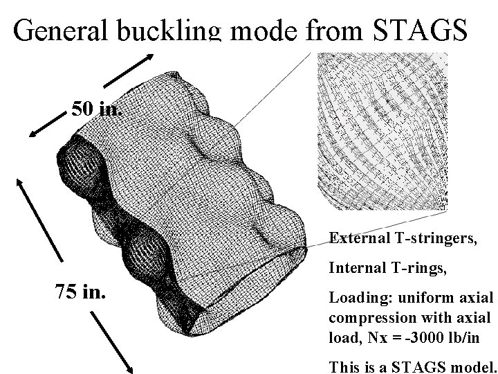
General buckling mode from STAGS 50 in. External T-stringers, Internal T-rings, 75 in. Loading: uniform axial compression with axial load, Nx = -3000 lb/in This is a STAGS model.

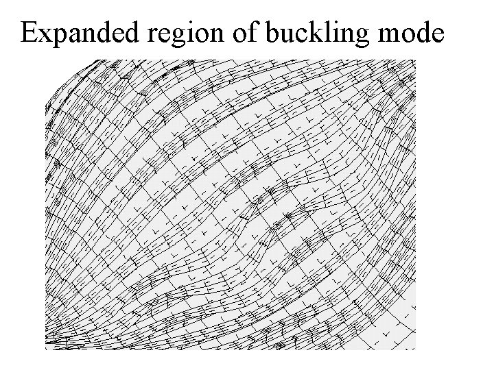
Expanded region of buckling mode

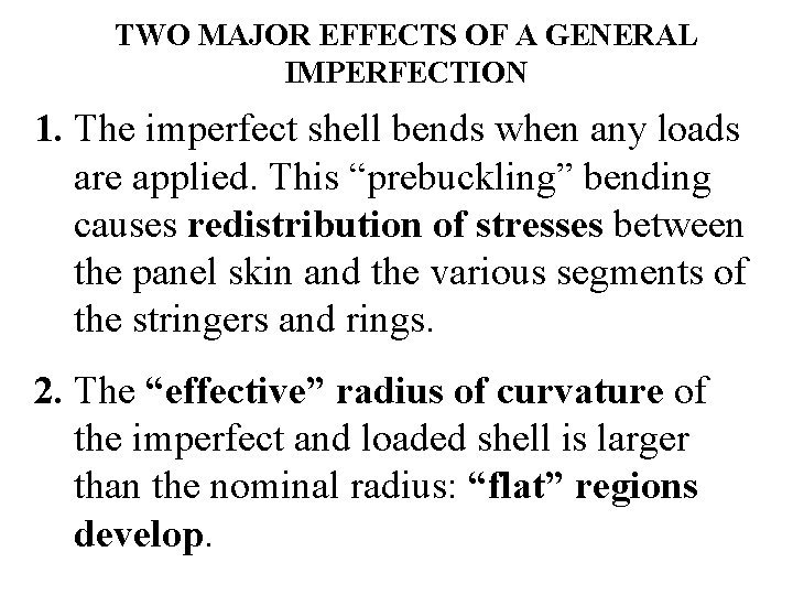
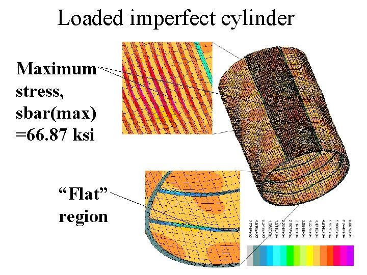
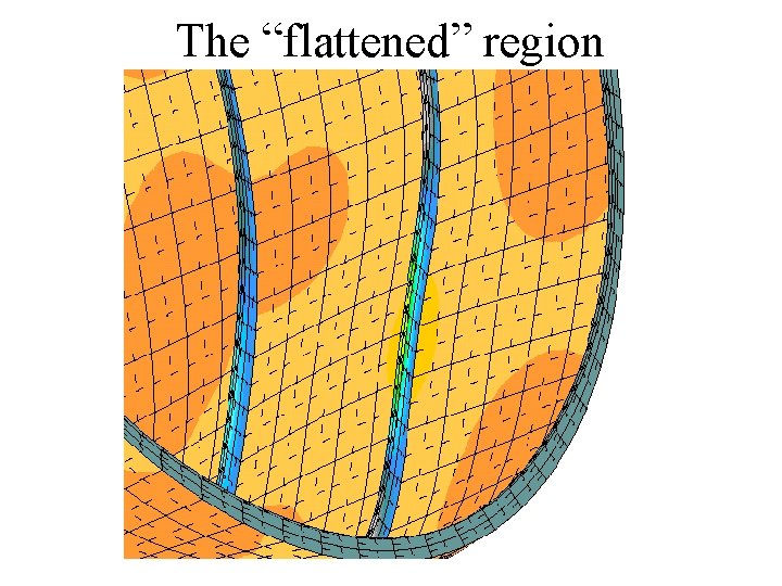
TWO MAJOR EFFECTS OF A GENERAL IMPERFECTION 1. The imperfect shell bends when any loads are applied. This “prebuckling” bending causes redistribution of stresses between the panel skin and the various segments of the stringers and rings. 2. The “effective” radius of curvature of the imperfect and loaded shell is larger than the nominal radius: “flat” regions develop.

Loaded imperfect cylinder Maximum stress, sbar(max) =66. 87 ksi “Flat” region

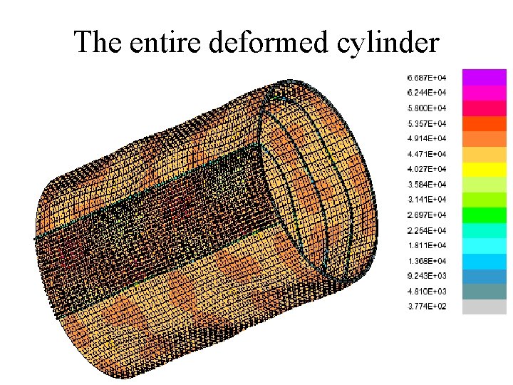
The entire deformed cylinder

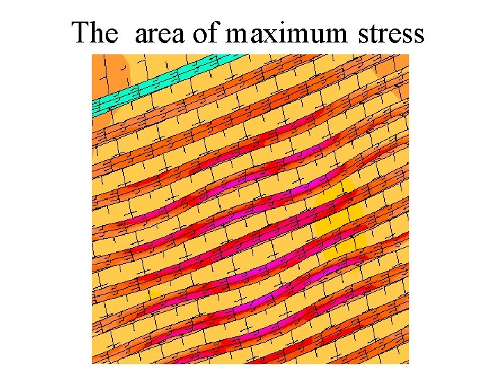
The area of maximum stress

The “flattened” region

Computer programs PANDA 2 and STAGS PANDA 2 optimizes ring and stringer stiffened flat or cylindrical panels and shells made of laminated composite material or simple isotropic or orthotropic material. The shells can be perfect or imperfect and can be loaded by up to five combinations of Nx, Ny Nxy. STAGS is a general-purpose program for the nonlinear elastic or elastic-plastic static and dynamic analyses. I used STAGS to check the optimum designs previously obtained by PANDA 2.

PHILOSOPHY OF PANDA 2 1. PANDA 2 obtains optimum designs through the use of many relatively simple models, each of which yields approximate buckling load factors (eigenvalues) and stresses. 2. 2. Details about these models are given in previous papers. Therefore, they are not repeated here. 3. 3. “Global” optimum designs can be obtained reasonably quickly and are not overly unconservative or conservative. 4. Because of the approximate nature of PANDA 2 models, optimum designs obtained by PANDA 2 should be checked by the use of a general-purpose finite element computer program. 5. STAGS is a good choice because PANDA 2 automatically generates input data for STAGS, and STAGS has excellent reliable nonlinear capabilities.

Example of PANDA 2 philosophy PANDA 2 computes general buckling from a simple closed-form model in which the stringers and rings are “smeared out” as prescribed by Baruch and Singer (1963). [Bushnell (1987)] Correction factors (knockdown factors) are computed to compensate for the inherent unconservativeness of this “smeared” model: one knockdown factor for “smearing” the stringers and another knockdown factor for “smearing” the rings. The next several slides demonstrate why a knockdown factor is needed to compensate for the inherent unconservativeness of “smearing” the rings and how this knockdown factor is computed.

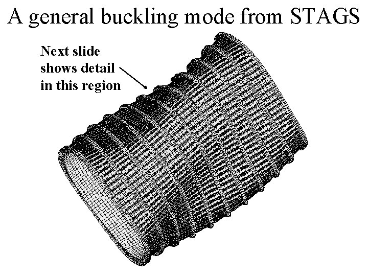
A general buckling mode from STAGS Next slide shows detail in this region

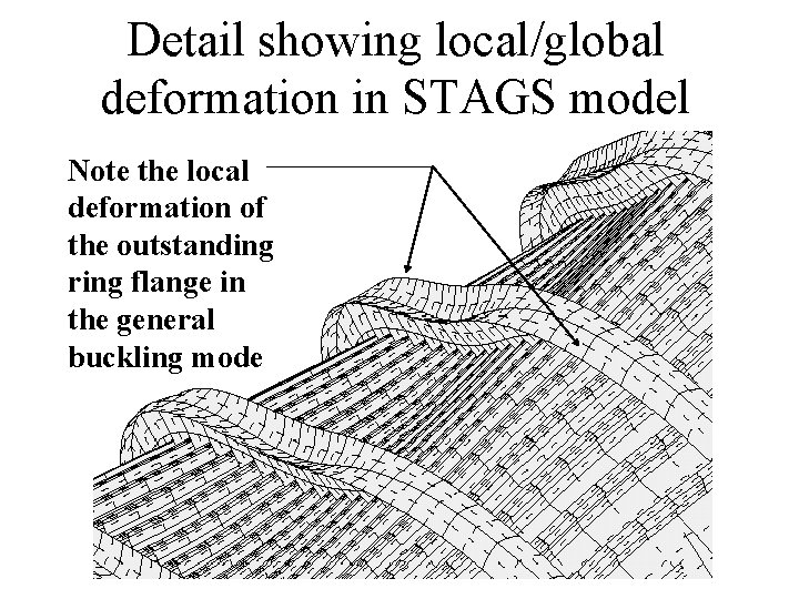
Detail showing local/global deformation in STAGS model Note the local deformation of the outstanding ring flange in the general buckling mode

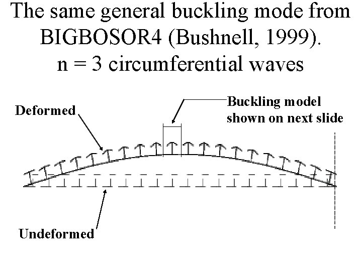
The same general buckling mode from BIGBOSOR 4 (Bushnell, 1999). n = 3 circumferential waves Deformed Undeformed Buckling model shown on next slide

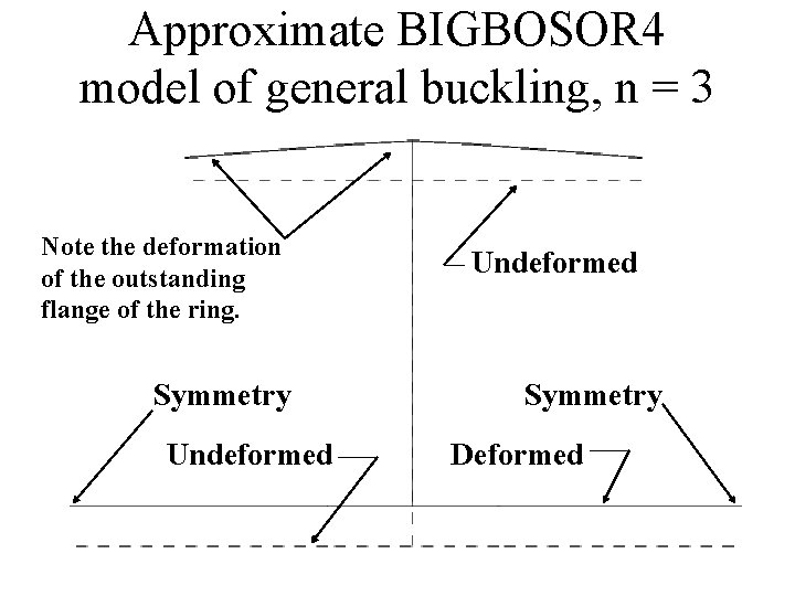
Approximate BIGBOSOR 4 model of general buckling, n = 3 Note the deformation of the outstanding flange of the ring. Symmetry Undeformed Symmetry Deformed

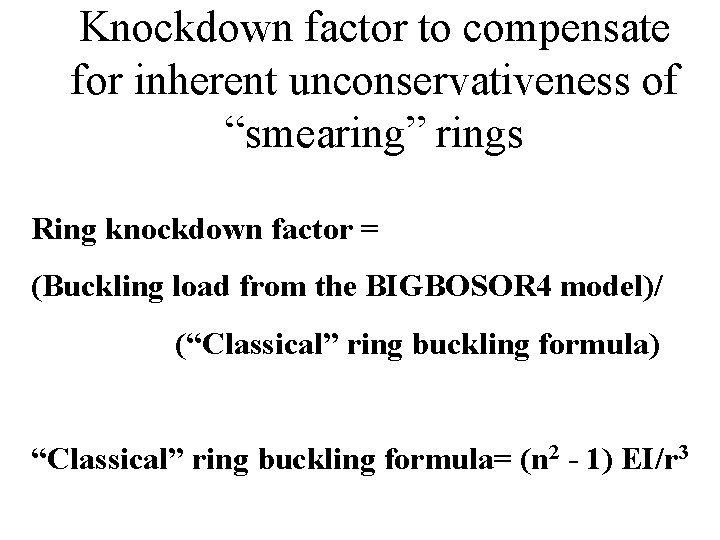
Knockdown factor to compensate for inherent unconservativeness of “smearing” rings Ring knockdown factor = (Buckling load from the BIGBOSOR 4 model)/ (“Classical” ring buckling formula) “Classical” ring buckling formula= (n 2 - 1) EI/r 3

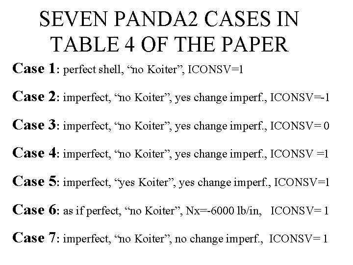
SEVEN PANDA 2 CASES IN TABLE 4 OF THE PAPER Case 1: perfect shell, “no Koiter”, ICONSV=1 Case 2: imperfect, “no Koiter”, yes change imperf. , ICONSV=-1 Case 3: imperfect, “no Koiter”, yes change imperf. , ICONSV= 0 Case 4: imperfect, “no Koiter”, yes change imperf. , ICONSV =1 Case 5: imperfect, “yes Koiter”, yes change imperf. , ICONSV=1 Case 6: as if perfect, “no Koiter”, Nx=-6000 lb/in, ICONSV= 1 Case 7: imperfect, “no Koiter”, no change imperf. , ICONSV= 1

Summary of talk 1. The configuration studied here 2. Two effects of a general imperfection 3. PANDA 2 and STAGS 4. PANDA 2 philosophy 5. Seven cases studied here 6. The optimization problem 7. Buckling and stress constraints 8. Seven cases explained 9. How the shells fail 10. Imperfection sensitivity

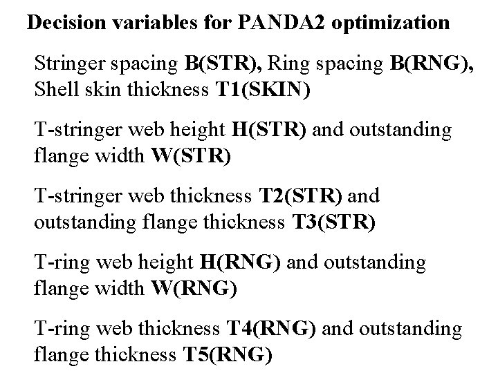
Decision variables for PANDA 2 optimization Stringer spacing B(STR), Ring spacing B(RNG), Shell skin thickness T 1(SKIN) T-stringer web height H(STR) and outstanding flange width W(STR) T-stringer web thickness T 2(STR) and outstanding flange thickness T 3(STR) T-ring web height H(RNG) and outstanding flange width W(RNG) T-ring web thickness T 4(RNG) and outstanding flange thickness T 5(RNG)

OBJECTIVE = MINIMUM WEIGHT

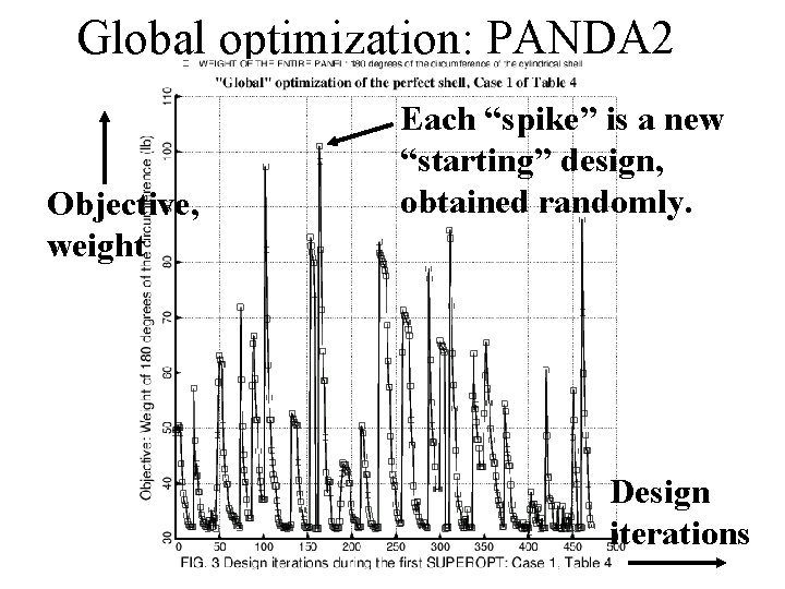
Global optimization: PANDA 2 Objective, weight Each “spike” is a new “starting” design, obtained randomly. Design iterations

CONSTRAINT CONDITIONS Five classes of constraint conditions: 1. Upper and lower bounds of decision variables 2. Linking conditions 3. Inequality constraints 4. Stress constraints 5. Buckling constraints

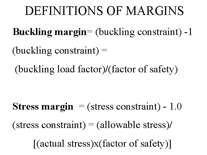
DEFINITIONS OF MARGINS Buckling margin= (buckling constraint) -1 (buckling constraint) = (buckling load factor)/(factor of safety) Stress margin = (stress constraint) - 1. 0 (stress constraint) = (allowable stress)/ [(actual stress)x(factor of safety)]

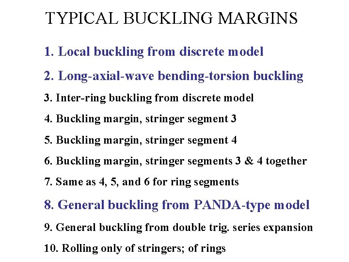
TYPICAL BUCKLING MARGINS 1. Local buckling from discrete model 2. Long-axial-wave bending-torsion buckling 3. Inter-ring buckling from discrete model 4. Buckling margin, stringer segment 3 5. Buckling margin, stringer segment 4 6. Buckling margin, stringer segments 3 & 4 together 7. Same as 4, 5, and 6 for ring segments 8. General buckling from PANDA-type model 9. General buckling from double trig. series expansion 10. Rolling only of stringers; of rings

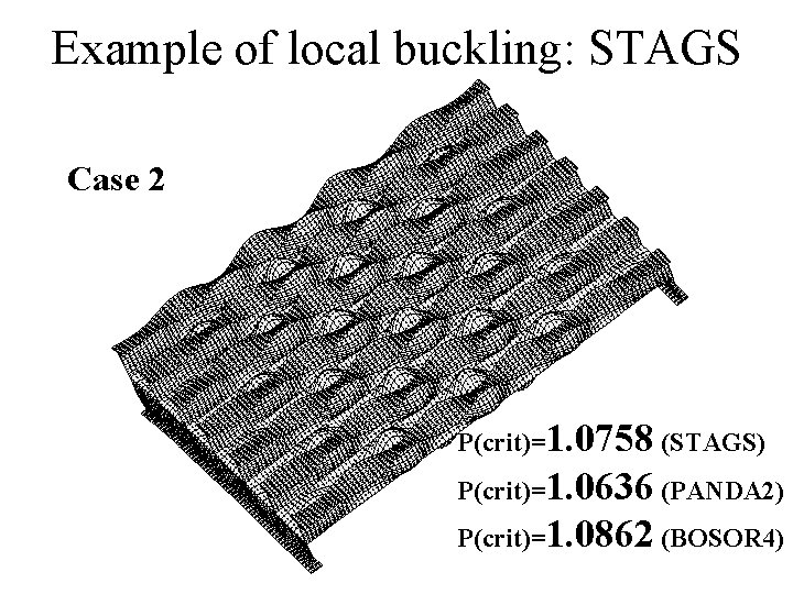
Example of local buckling: STAGS Case 2 P(crit)=1. 0758 (STAGS) P(crit)=1. 0636 (PANDA 2) P(crit)=1. 0862 (BOSOR 4)

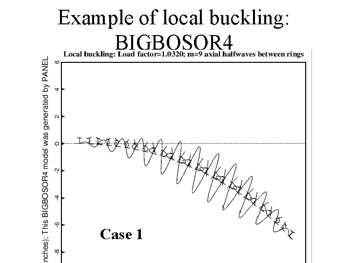
Example of local buckling: BIGBOSOR 4 Case 1

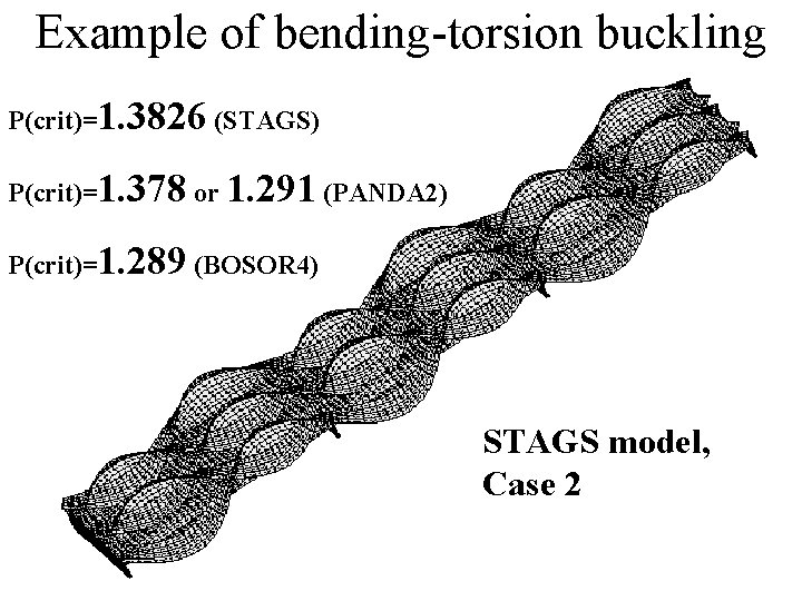
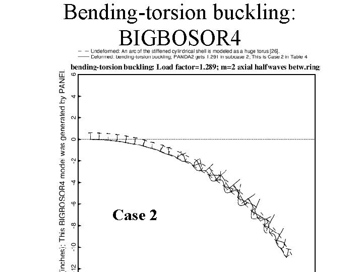
Example of bending-torsion buckling P(crit)=1. 3826 (STAGS) P(crit)=1. 378 or 1. 291 (PANDA 2) P(crit)=1. 289 (BOSOR 4) STAGS model, Case 2

Bending-torsion buckling: BIGBOSOR 4 Case 2

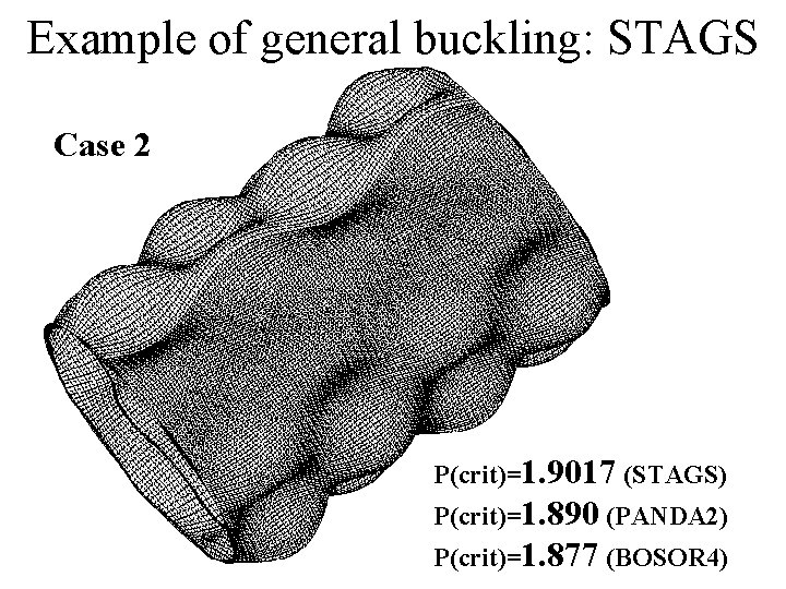
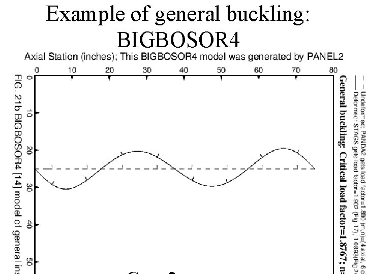
Example of general buckling: STAGS Case 2 P(crit)=1. 9017 (STAGS) P(crit)=1. 890 (PANDA 2) P(crit)=1. 877 (BOSOR 4)

Example of general buckling: BIGBOSOR 4

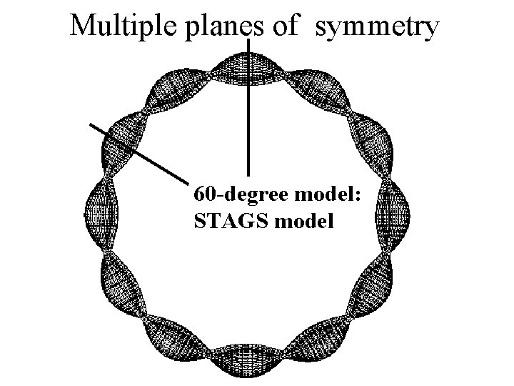
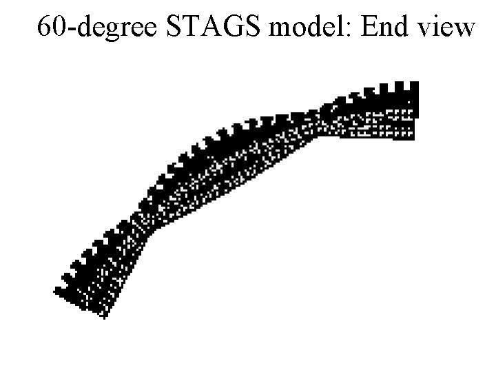
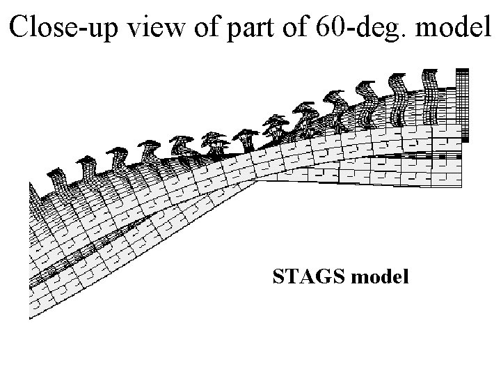
Multiple planes of symmetry 60 -degree model: STAGS model

60 -degree STAGS model: End view

Close-up view of part of 60 -deg. model STAGS model

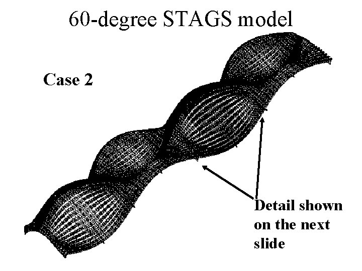
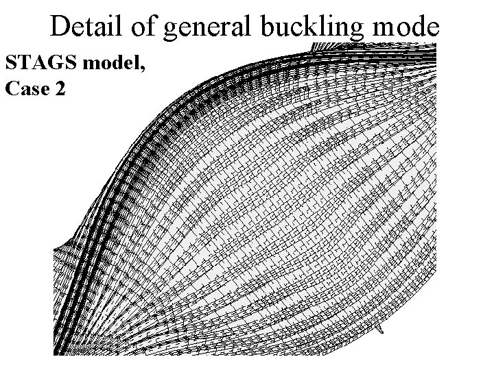
60 -degree STAGS model Case 2 Detail shown on the next slide

Detail of general buckling mode STAGS model, Case 2

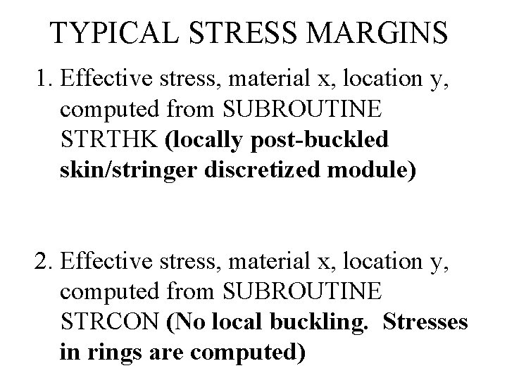
TYPICAL STRESS MARGINS 1. Effective stress, material x, location y, computed from SUBROUTINE STRTHK (locally post-buckled skin/stringer discretized module) 2. Effective stress, material x, location y, computed from SUBROUTINE STRCON (No local buckling. Stresses in rings are computed)

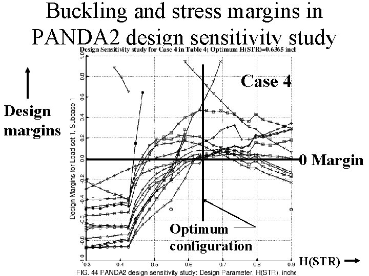
Buckling and stress margins in PANDA 2 design sensitivity study Case 4 Design margins 0 Margin Optimum configuration H(STR)

Summary of talk 1. The configuration studied here 2. Two effects of a general imperfection 3. PANDA 2 and STAGS 4. PANDA 2 philosophy 5. Seven cases studied here 6. The optimization problem 7. Buckling and stress constraints 8. Seven cases explained 9. How the shells fail 10. Imperfection sensitivity

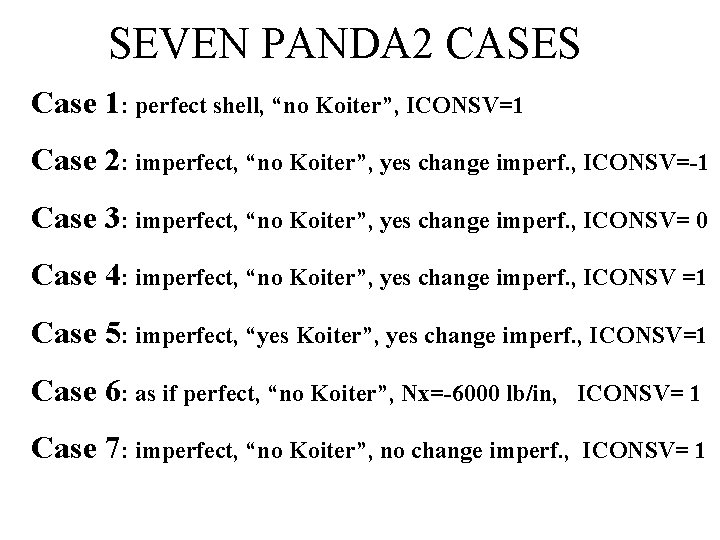
SEVEN PANDA 2 CASES Case 1: perfect shell, “no Koiter”, ICONSV=1 Case 2: imperfect, “no Koiter”, yes change imperf. , ICONSV=-1 Case 3: imperfect, “no Koiter”, yes change imperf. , ICONSV= 0 Case 4: imperfect, “no Koiter”, yes change imperf. , ICONSV =1 Case 5: imperfect, “yes Koiter”, yes change imperf. , ICONSV=1 Case 6: as if perfect, “no Koiter”, Nx=-6000 lb/in, ICONSV= 1 Case 7: imperfect, “no Koiter”, no change imperf. , ICONSV= 1

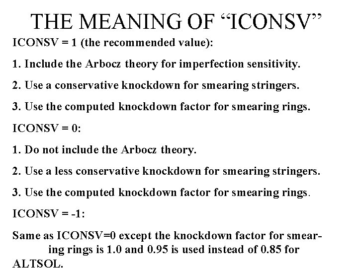
THE MEANING OF “ICONSV” ICONSV = 1 (the recommended value): 1. Include the Arbocz theory for imperfection sensitivity. 2. Use a conservative knockdown for smearing stringers. 3. Use the computed knockdown factor for smearings. ICONSV = 0: 1. Do not include the Arbocz theory. 2. Use a less conservative knockdown for smearing stringers. 3. Use the computed knockdown factor for smearings. ICONSV = -1: Same as ICONSV=0 except the knockdown factor for smearings is 1. 0 and 0. 95 is used instead of 0. 85 for ALTSOL.

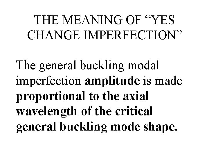
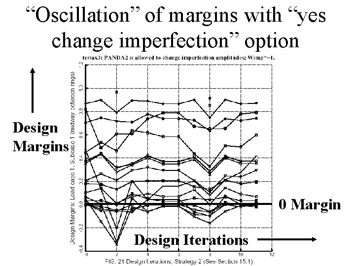
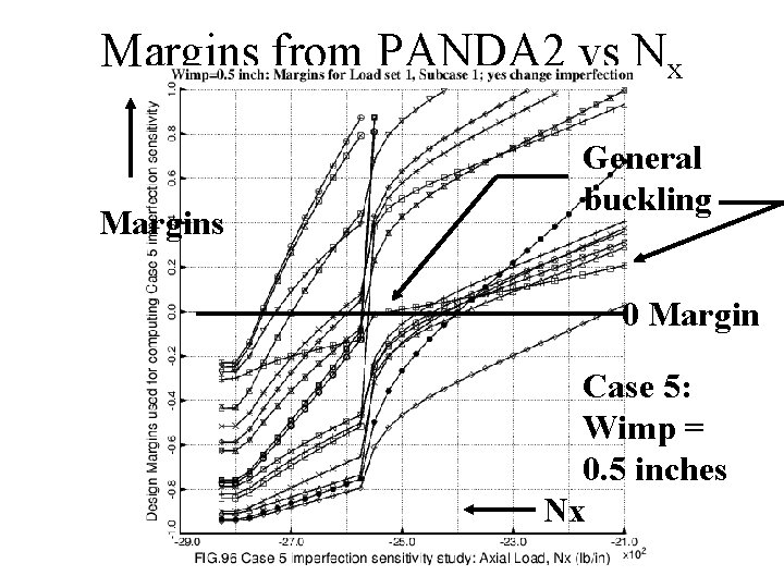
THE MEANING OF “YES CHANGE IMPERFECTION” The general buckling modal imperfection amplitude is made proportional to the axial wavelength of the critical general buckling mode shape.

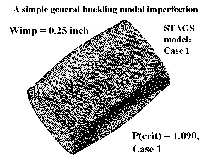
A simple general buckling modal imperfection Wimp = 0. 25 inch STAGS model: Case 1 P(crit) = 1. 090, Case 1

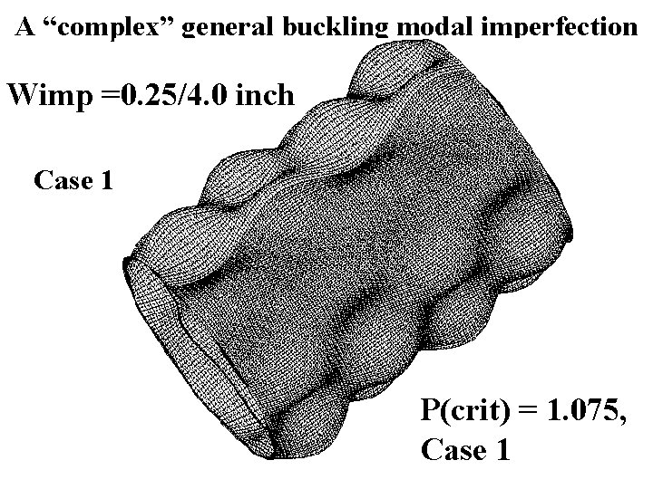
A “complex” general buckling modal imperfection Wimp =0. 25/4. 0 inch Case 1 P(crit) = 1. 075, Case 1

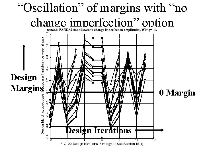
“Oscillation” of margins with “no change imperfection” option Design Margins 0 Margin Design Iterations

“Oscillation” of margins with “yes change imperfection” option Design Margins 0 Margin Design Iterations

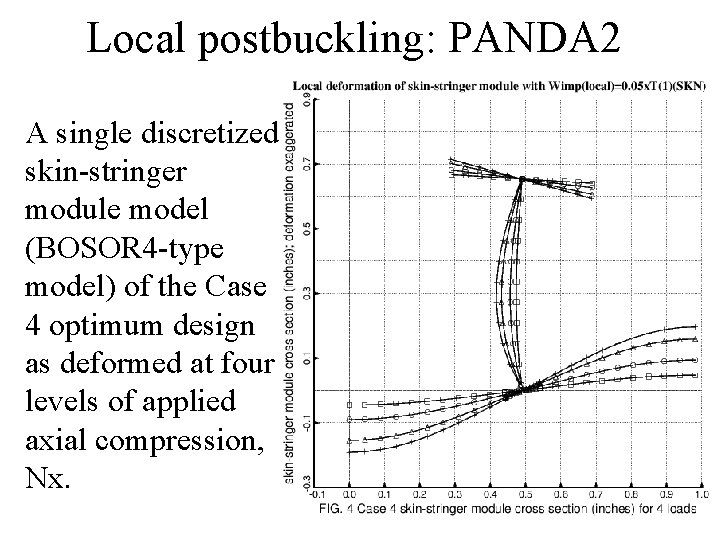
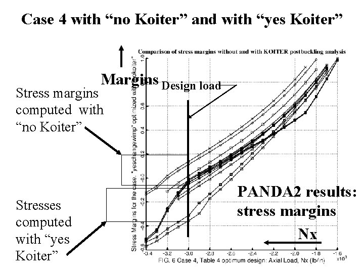
THE MEANING OF “NO” AND “YES KOITER” “NO KOITER” = no local postbuckling state is computed. “YES KOITER” = the local postbuckling state is computed. A modified form of the nonlinear theory by KOITER (1946), BUSHNELL (1993) is used.

Local postbuckling: PANDA 2 A single discretized skin-stringer module model (BOSOR 4 -type model) of the Case 4 optimum design as deformed at four levels of applied axial compression, Nx.

Case 4 with “no Koiter” and with “yes Koiter” Margins Design load Stress margins computed with “no Koiter” Stresses computed with “yes Koiter” PANDA 2 results: stress margins Nx

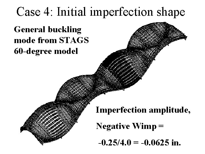
Case 4: Initial imperfection shape General buckling mode from STAGS 60 -degree model Imperfection amplitude, Negative Wimp = -0. 25/4. 0 = -0. 0625 in.

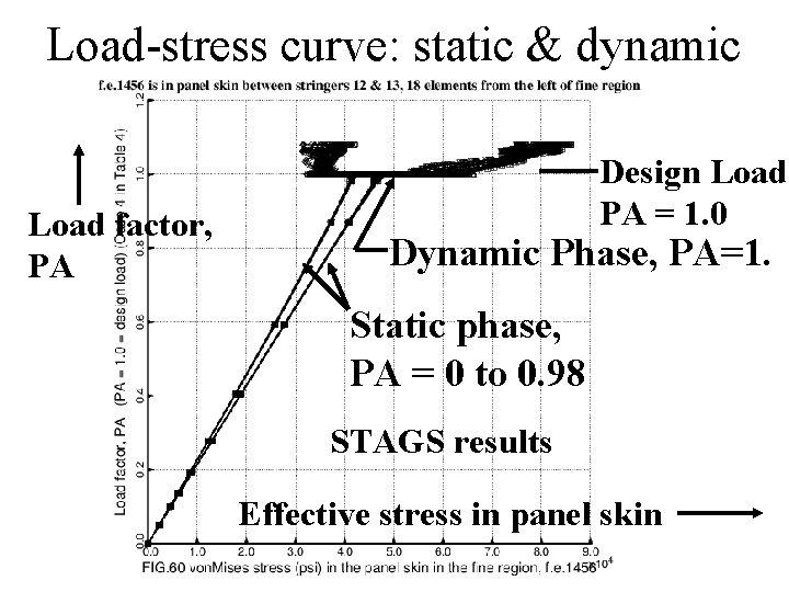
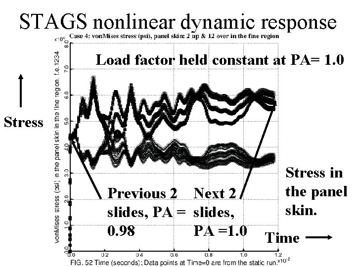
Load-stress curve: static & dynamic Load factor, PA Design Load, PA = 1. 0 Dynamic Phase, PA=1. Static phase, PA = 0 to 0. 98 STAGS results Effective stress in panel skin

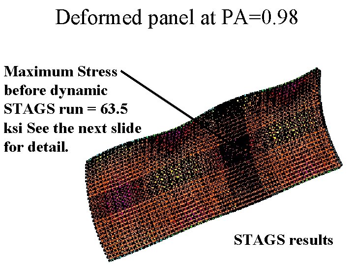
Deformed panel at PA=0. 98 Maximum Stress before dynamic STAGS run = 63. 5 ksi See the next slide for detail. STAGS results

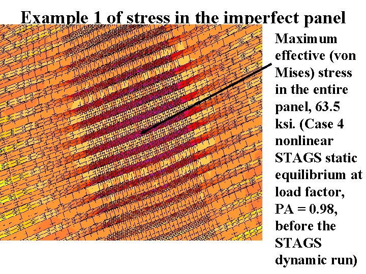
Example 1 of stress in the imperfect panel Maximum effective (von Mises) stress in the entire panel, 63. 5 ksi. (Case 4 nonlinear STAGS static equilibrium at load factor, PA = 0. 98, before the STAGS dynamic run)

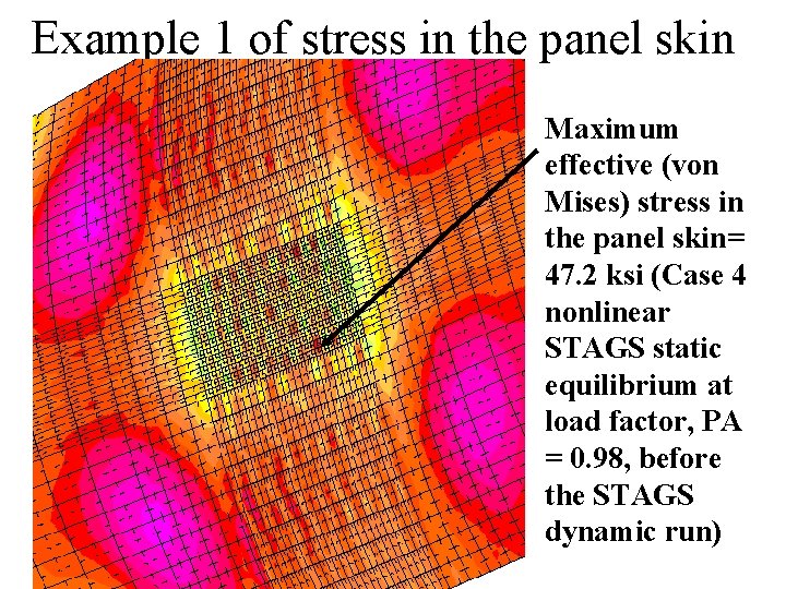
Example 1 of stress in the panel skin Maximum effective (von Mises) stress in the panel skin= 47. 2 ksi (Case 4 nonlinear STAGS static equilibrium at load factor, PA = 0. 98, before the STAGS dynamic run)

STAGS nonlinear dynamic response Load factor held constant at PA= 1. 0 Stress Previous 2 Next 2 slides, PA = slides, 0. 98 PA =1. 0 Stress in the panel skin. Time

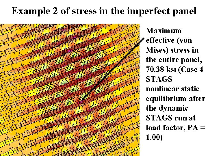
Example 2 of stress in the imperfect panel Maximum effective (von Mises) stress in the entire panel, 70. 38 ksi (Case 4 STAGS nonlinear static equilibrium after the dynamic STAGS run at load factor, PA = 1. 00)

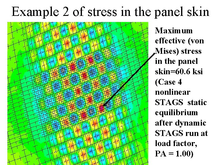
Example 2 of stress in the panel skin Maximum effective (von Mises) stress in the panel skin=60. 6 ksi (Case 4 nonlinear STAGS static equilibrium after dynamic STAGS run at load factor, PA = 1. 00)

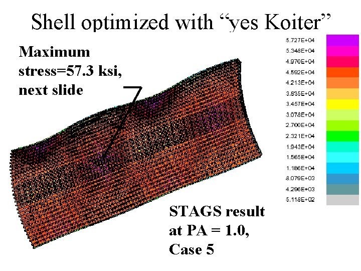
Shell optimized with “yes Koiter” Maximum stress=57. 3 ksi, next slide STAGS result at PA = 1. 0, Case 5

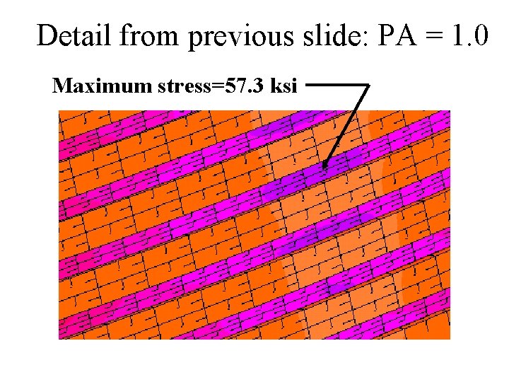
Detail from previous slide: PA = 1. 0 Maximum stress=57. 3 ksi

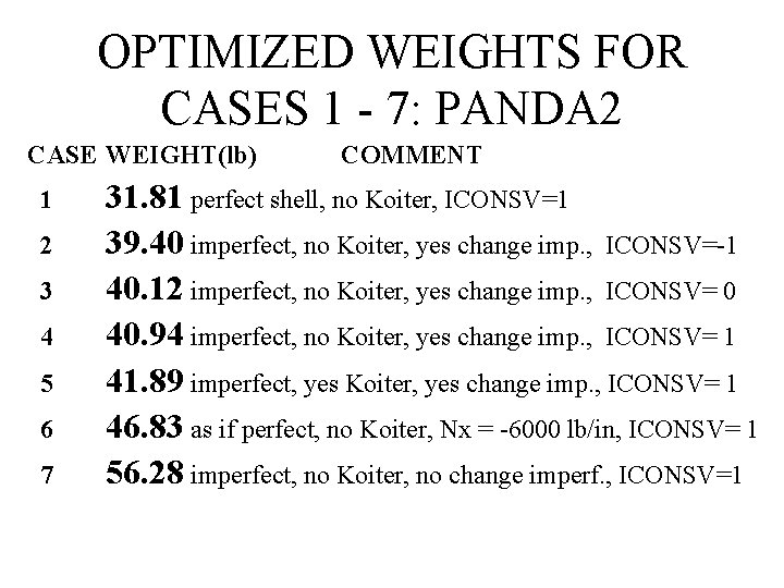
OPTIMIZED WEIGHTS FOR CASES 1 - 7: PANDA 2 CASE WEIGHT(lb) 1 2 3 4 5 6 7 COMMENT 31. 81 perfect shell, no Koiter, ICONSV=1 39. 40 imperfect, no Koiter, yes change imp. , ICONSV=-1 40. 12 imperfect, no Koiter, yes change imp. , ICONSV= 0 40. 94 imperfect, no Koiter, yes change imp. , ICONSV= 1 41. 89 imperfect, yes Koiter, yes change imp. , ICONSV= 1 46. 83 as if perfect, no Koiter, Nx = -6000 lb/in, ICONSV= 1 56. 28 imperfect, no Koiter, no change imperf. , ICONSV=1

Summary of talk 1. The configuration studied here 2. Two effects of a general imperfection 3. PANDA 2 and STAGS 4. PANDA 2 philosophy 5. Seven cases studied here 6. The optimization problem 7. Buckling and stress constraints 8. Seven cases explained 9. How the shells fail 10. Imperfection sensitivity

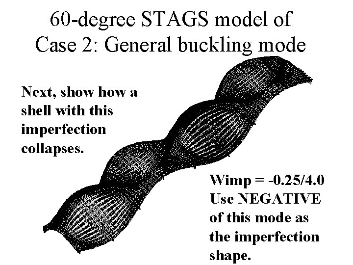
60 -degree STAGS model of Case 2: General buckling mode Next, show a shell with this imperfection collapses. Wimp = -0. 25/4. 0 Use NEGATIVE of this mode as the imperfection shape.

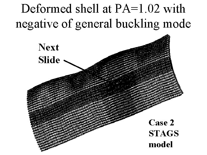
Deformed shell at PA=1. 02 with negative of general buckling mode Next Slide Case 2 STAGS model

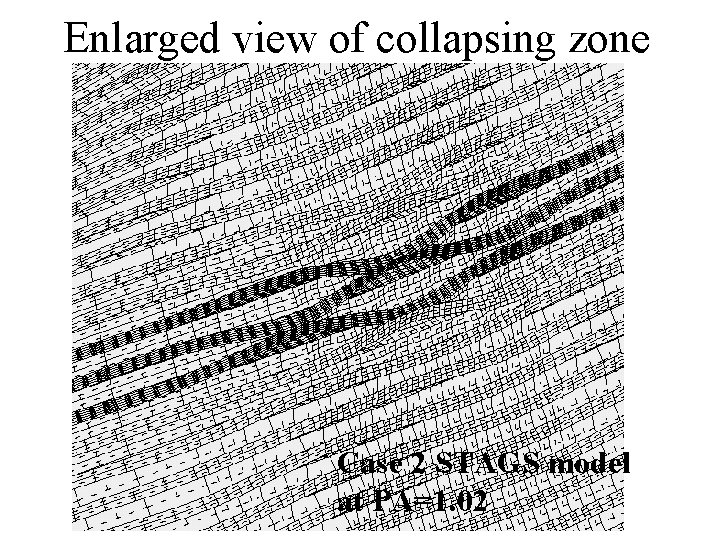
Enlarged view of collapsing zone Case 2 STAGS model at PA=1. 02

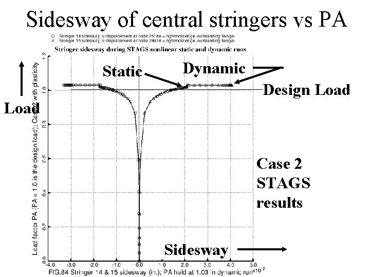
Sidesway of central stringers vs PA Static Dynamic Design Load Case 2 STAGS results Sidesway

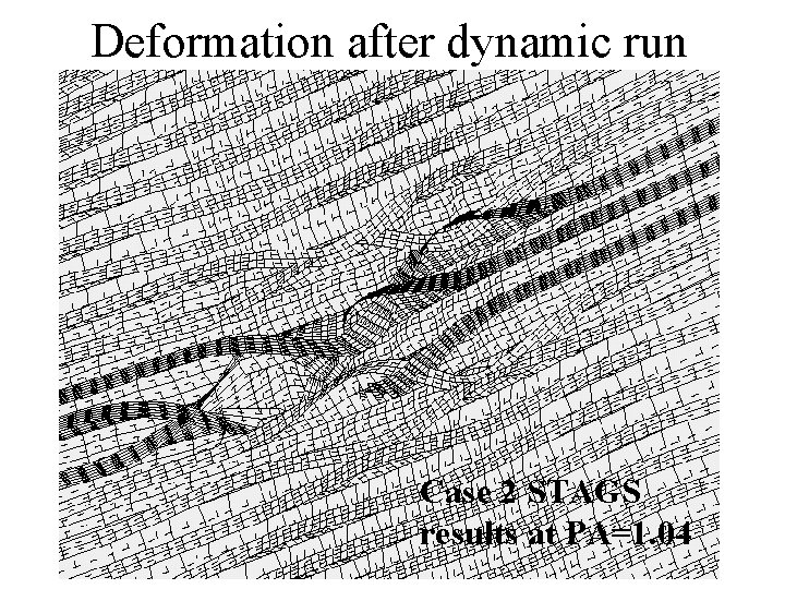
Deformation after dynamic run Case 2 STAGS results at PA=1. 04

Summary of talk 1. The configuration studied here 2. Two effects of a general imperfection 3. PANDA 2 and STAGS 4. PANDA 2 philosophy 5. Seven cases studied here 6. The optimization problem 7. Buckling and stress constraints 8. Seven cases explained 9. How the shells fail 10. Imperfection sensitivity

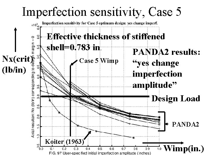
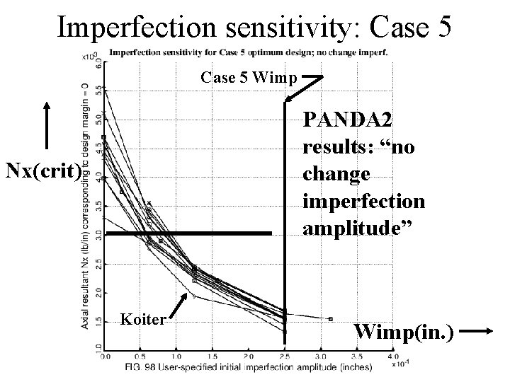
Imperfection sensitivity, Case 5 Nx(crit) (lb/in) Effective thickness of stiffened shell=0. 783 in. PANDA 2 results: Case 5 Wimp “yes change imperfection amplitude” Design Load PANDA 2 Koiter (1963) Wimp(in. )

Margins from PANDA 2 vs Nx Margins General buckling 0 Margin Case 5: Wimp = 0. 5 inches Nx

Imperfection sensitivity: Case 5 Wimp PANDA 2 results: “no change imperfection amplitude” Nx(crit) Koiter Wimp(in. )

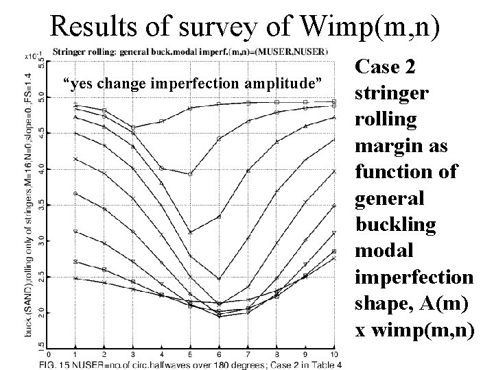
Results of survey of Wimp(m, n) “yes change imperfection amplitude” Case 2 stringer rolling margin as function of general buckling modal imperfection shape, A(m) x wimp(m, n)

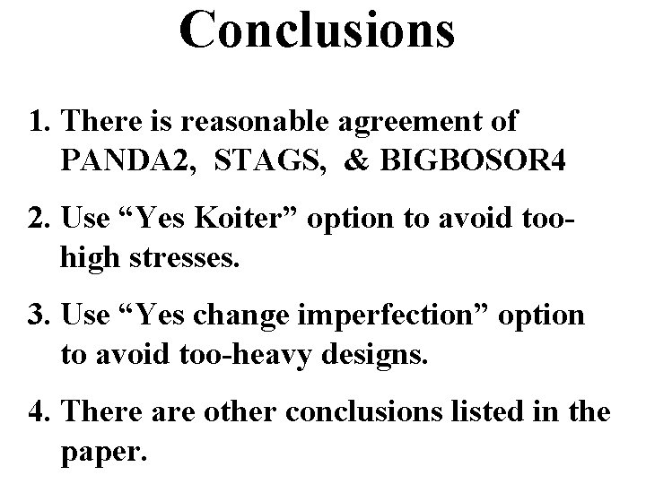
Conclusions 1. There is reasonable agreement of PANDA 2, STAGS, & BIGBOSOR 4 2. Use “Yes Koiter” option to avoid toohigh stresses. 3. Use “Yes change imperfection” option to avoid too-heavy designs. 4. There are other conclusions listed in the paper.