Numpy Arrays Num Py Fancy Indexing Fancy indexing

Numpy Arrays

Num. Py: Fancy Indexing • Fancy indexing: • Use an array of indices in order to access a number of array elements at once

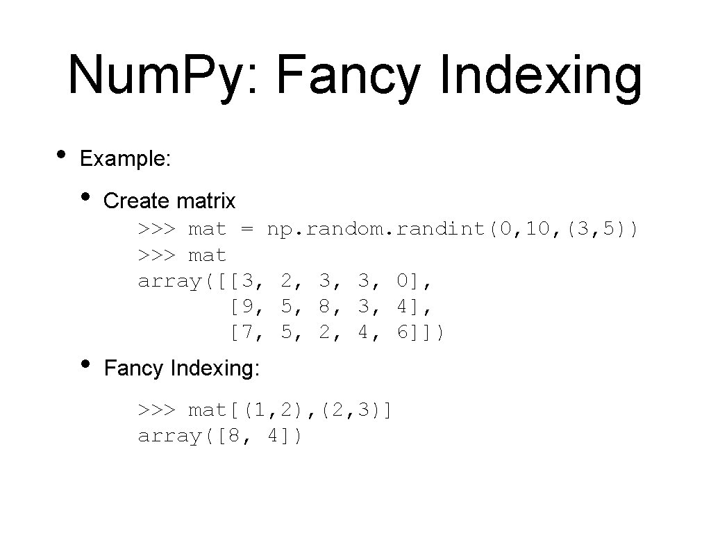
Num. Py: Fancy Indexing • Example: • Create matrix >>> mat = np. random. randint(0, 10, (3, 5)) >>> mat array([[3, 2, 3, 3, 0], [9, 5, 8, 3, 4], [7, 5, 2, 4, 6]]) • Fancy Indexing: >>> mat[(1, 2), (2, 3)] array([8, 4])

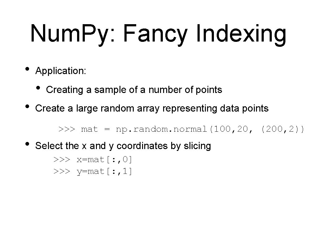
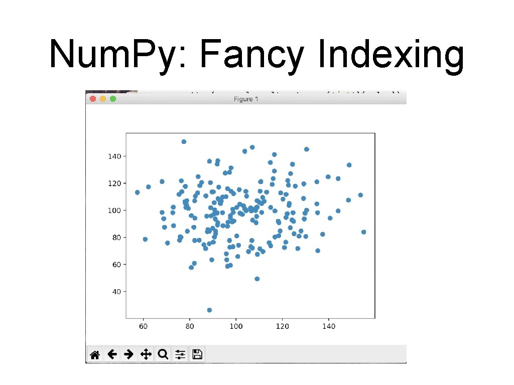
Num. Py: Fancy Indexing • Application: • • Creating a sample of a number of points Create a large random array representing data points >>> mat = np. random. normal(100, 20, (200, 2)) • Select the x and y coordinates by slicing >>> x=mat[: , 0] >>> y=mat[: , 1]

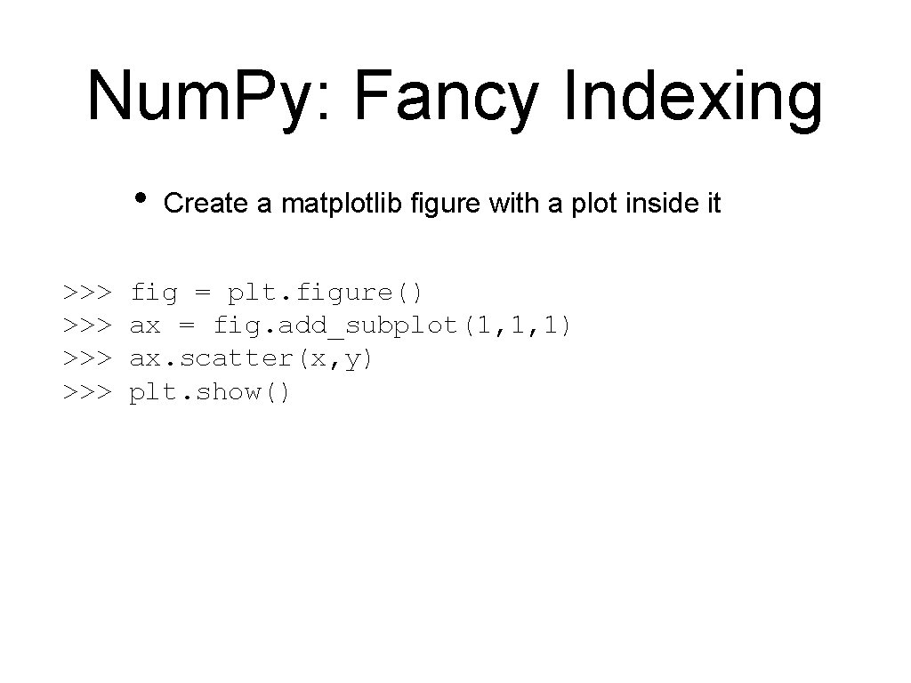
Num. Py: Fancy Indexing • >>> >>> Create a matplotlib figure with a plot inside it fig = plt. figure() ax = fig. add_subplot(1, 1, 1) ax. scatter(x, y) plt. show()

Num. Py: Fancy Indexing

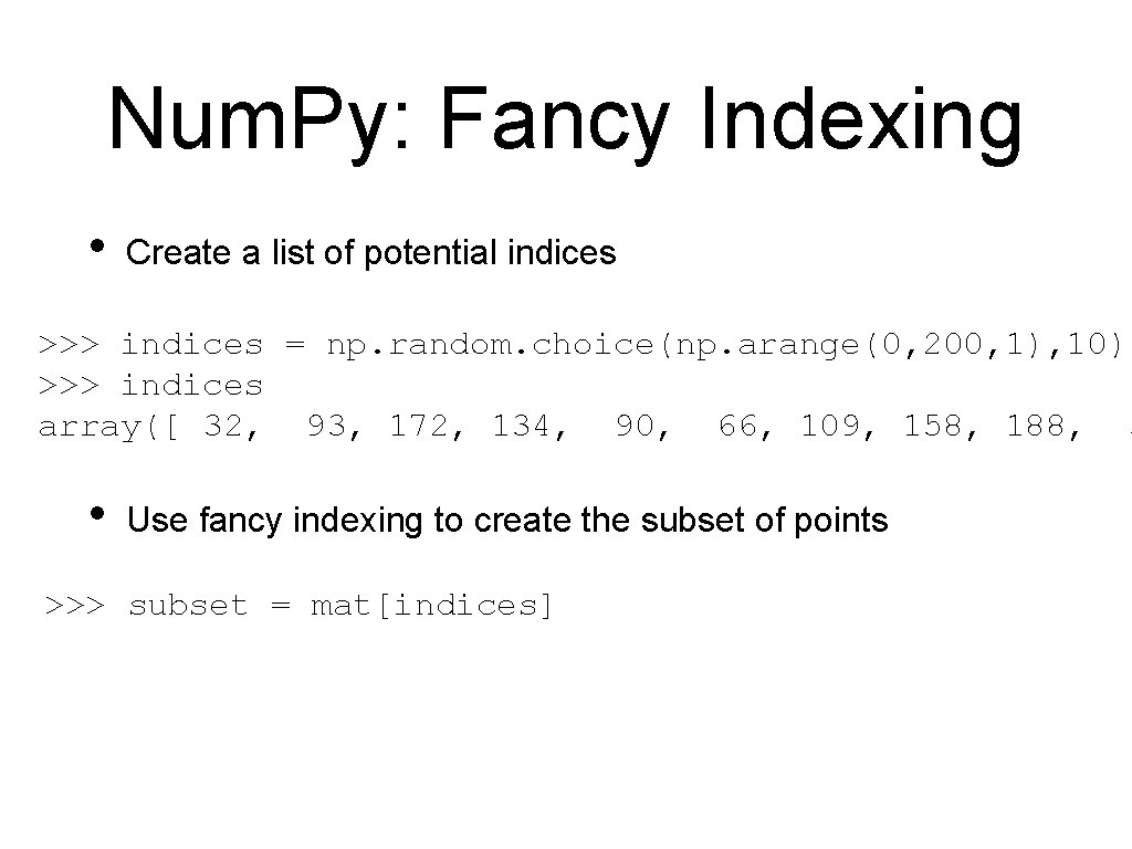
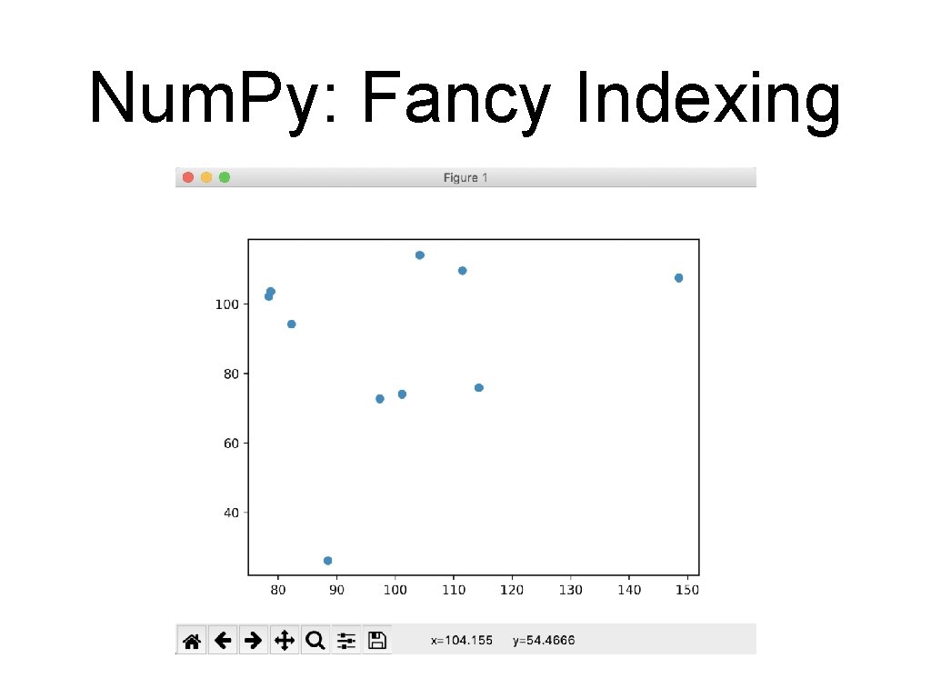
Num. Py: Fancy Indexing • Create a list of potential indices >>> indices = np. random. choice(np. arange(0, 200, 1), 10) >>> indices array([ 32, 93, 172, 134, 90, 66, 109, 158, 188, 3 • Use fancy indexing to create the subset of points >>> subset = mat[indices]

Num. Py: Fancy Indexing

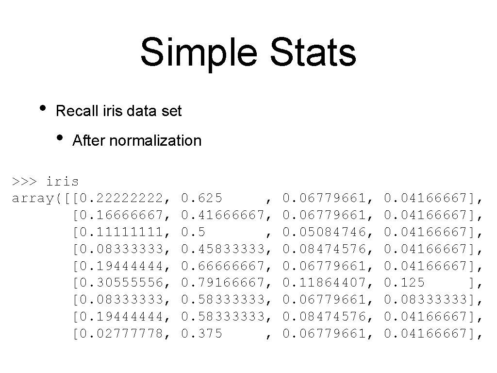
Simple Stats • Recall iris data set • After normalization >>> iris array([[0. 2222, [0. 16666667, [0. 1111, [0. 08333333, [0. 19444444, [0. 30555556, [0. 08333333, [0. 19444444, [0. 02777778, 0. 625 , 0. 41666667, 0. 5 , 0. 45833333, 0. 66666667, 0. 79166667, 0. 58333333, 0. 375 , 0. 06779661, 0. 05084746, 0. 08474576, 0. 06779661, 0. 11864407, 0. 06779661, 0. 08474576, 0. 06779661, 0. 04166667], 0. 125 ], 0. 08333333], 0. 04166667],

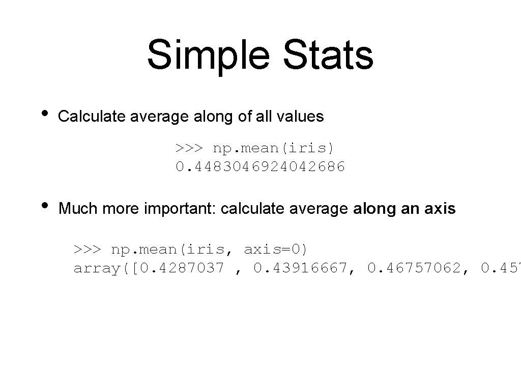
Simple Stats • Calculate average along of all values >>> np. mean(iris) 0. 4483046924042686 • Much more important: calculate average along an axis >>> np. mean(iris, axis=0) array([0. 4287037 , 0. 43916667, 0. 46757062, 0. 457

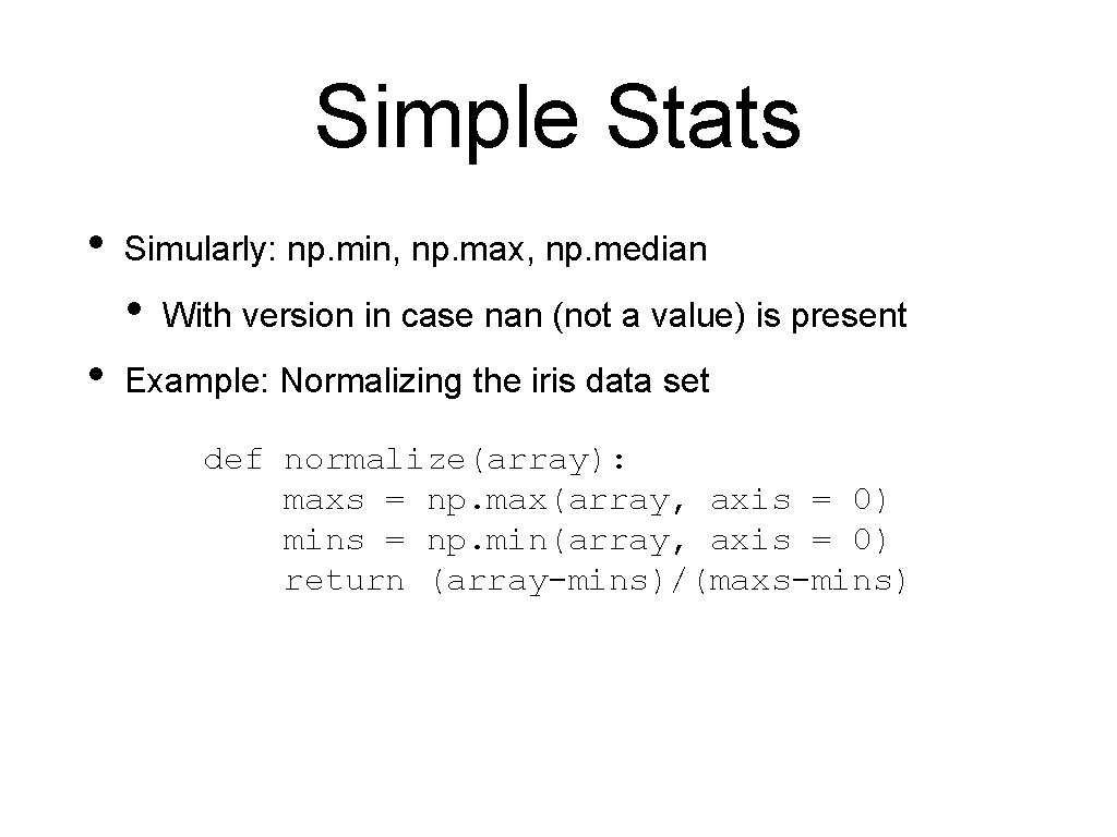
Simple Stats • Simularly: np. min, np. max, np. median • • With version in case nan (not a value) is present Example: Normalizing the iris data set def normalize(array): maxs = np. max(array, axis = 0) mins = np. min(array, axis = 0) return (array-mins)/(maxs-mins)

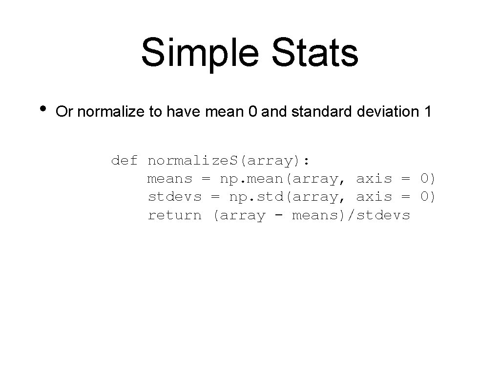
Simple Stats • Or normalize to have mean 0 and standard deviation 1 def normalize. S(array): means = np. mean(array, axis = 0) stdevs = np. std(array, axis = 0) return (array - means)/stdevs

Simple Stats • Can determine percentiles and quantiles >>> iris[: 5, : ] array([[5. 1, 3. 5, 1. 4, 0. 2], [4. 9, 3. , 1. 4, 0. 2], [4. 7, 3. 2, 1. 3, 0. 2], [4. 6, 3. 1, 1. 5, 0. 2], [5. , 3. 6, 1. 4, 0. 2]]) ]) >>> np. percentile(iris, 5, axis=0) array([4. 6 , 2. 345, 1. 3 , 0. 2 ]) np. percentile(iris, 95, axis=0) array([7. 255, 3. 8 , 6. 1 , 2. 3 ])

Broadcast Application • Getting the difference matrix of a vector

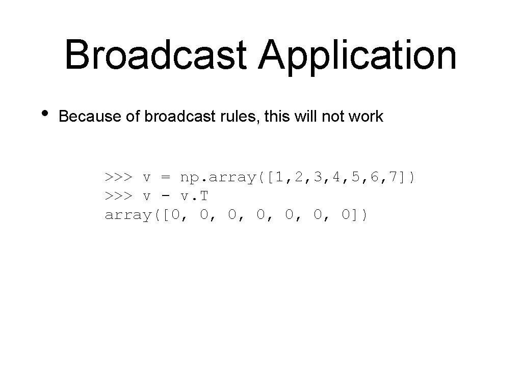
Broadcast Application • Because of broadcast rules, this will not work >>> v = np. array([1, 2, 3, 4, 5, 6, 7]) >>> v - v. T array([0, 0, 0, 0])

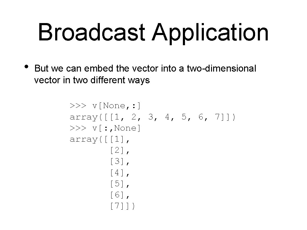
Broadcast Application • But we can embed the vector into a two-dimensional vector in two different ways >>> v[None, : ] array([[1, 2, 3, 4, 5, 6, 7]]) >>> v[: , None] array([[1], [2], [3], [4], [5], [6], [7]])

Broadcast Application • Now we can use broadcasting >>> v[: , None]-v[None, : ] array([[ 0, -1, -2, -3, [ 1, 0, -1, -2, [ 2, 1, 0, -1, [ 3, 2, 1, 0, [ 4, 3, 2, 1, [ 5, 4, 3, 2, [ 6, 5, 4, 3, -4, -3, -2, -1, 0, 1, 2, -5, -4, -3, -2, -1, 0, 1, -6], -5], -4], -3], -2], -1], 0]])

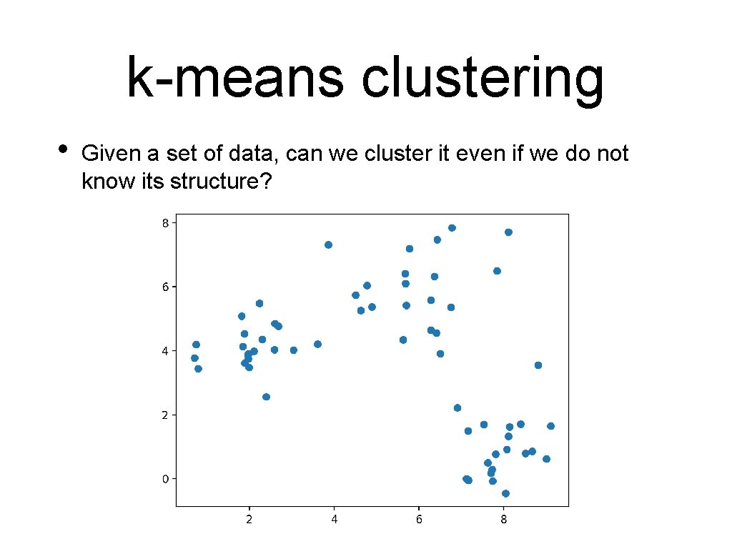
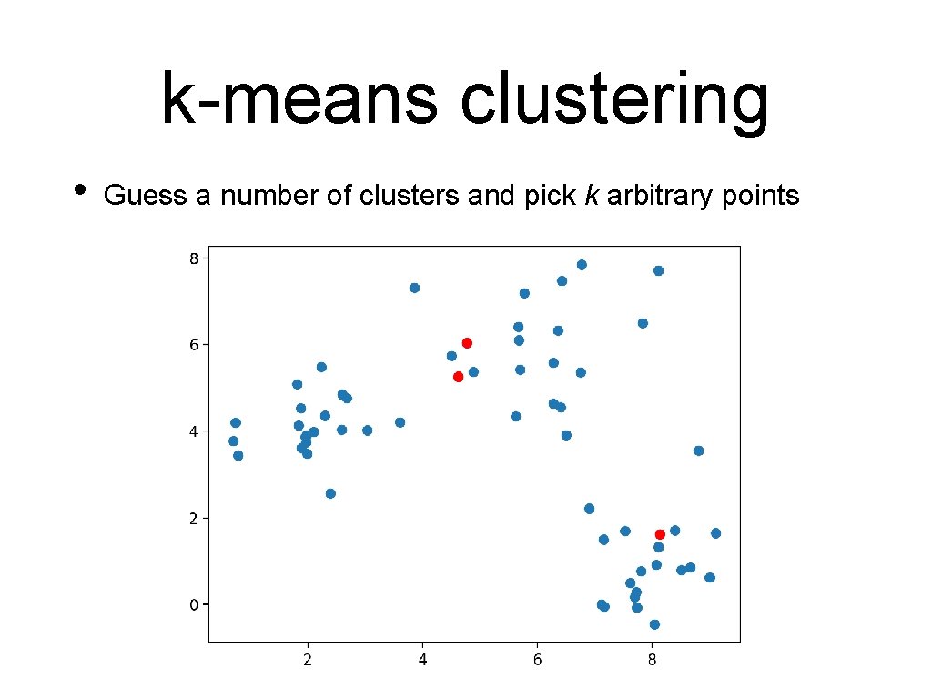
k-means clustering • Given a set of data, can we cluster it even if we do not know its structure?

k-means clustering • Guess a number of clusters and pick k arbitrary points

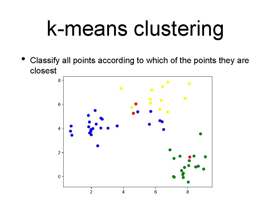
k-means clustering • Classify all points according to which of the points they are closest

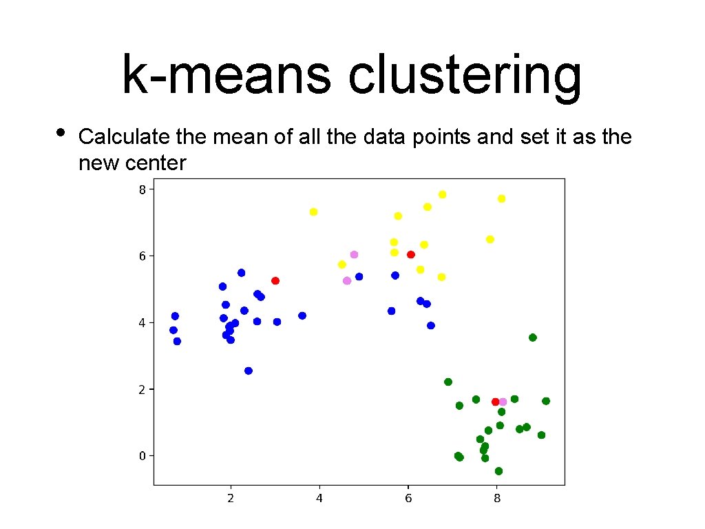
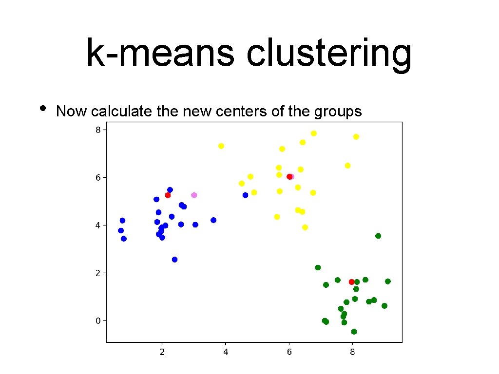
k-means clustering • Calculate the mean of all the data points and set it as the new center

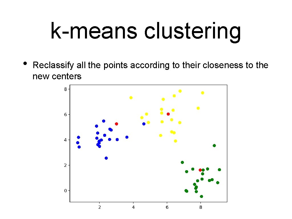
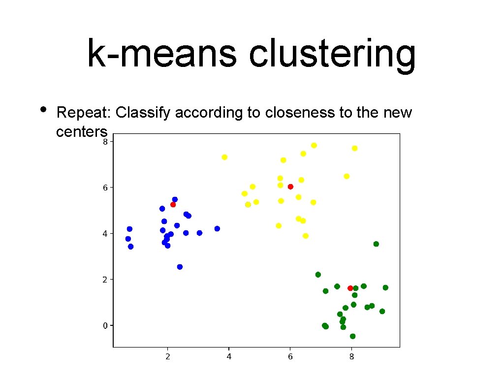
k-means clustering • Reclassify all the points according to their closeness to the new centers

k-means clustering • Now calculate the new centers of the groups

k-means clustering • Repeat: Classify according to closeness to the new centers

k-means clustering • Continue • The centers no longer move when points are no longer moved between different categories

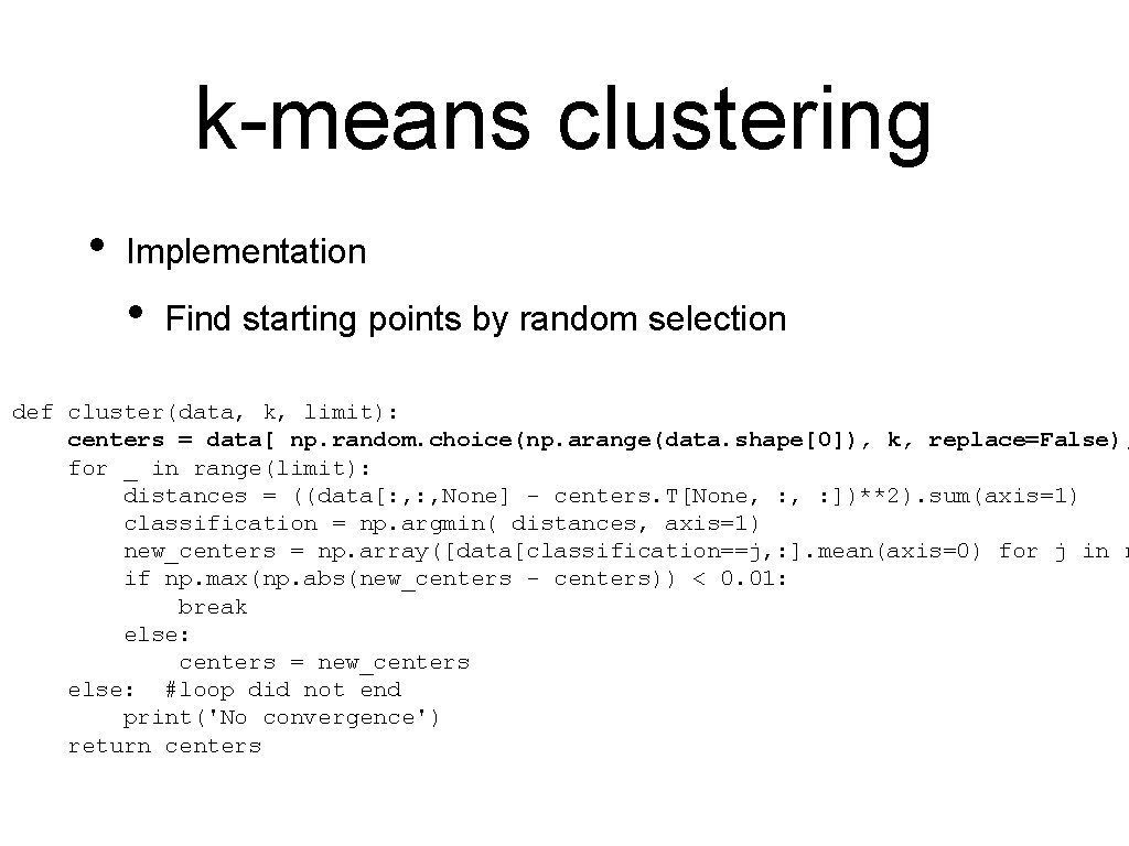
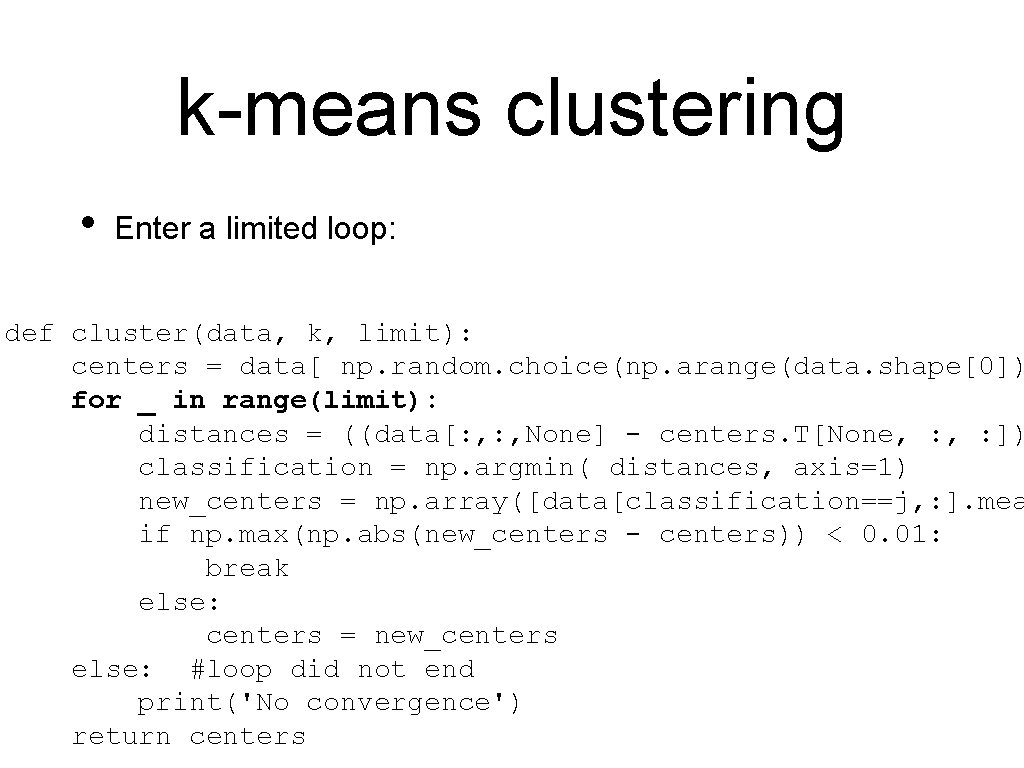
k-means clustering • Implementation • Find starting points by random selection def cluster(data, k, limit): centers = data[ np. random. choice(np. arange(data. shape[0]), k, replace=False), for _ in range(limit): distances = ((data[: , None] - centers. T[None, : ])**2). sum(axis=1) classification = np. argmin( distances, axis=1) new_centers = np. array([data[classification==j, : ]. mean(axis=0) for j in r if np. max(np. abs(new_centers - centers)) < 0. 01: break else: centers = new_centers else: #loop did not end print('No convergence') return centers

k-means clustering • Enter a limited loop: def cluster(data, k, limit): centers = data[ np. random. choice(np. arange(data. shape[0]) for _ in range(limit): distances = ((data[: , None] - centers. T[None, : ]) classification = np. argmin( distances, axis=1) new_centers = np. array([data[classification==j, : ]. mea if np. max(np. abs(new_centers - centers)) < 0. 01: break else: centers = new_centers else: #loop did not end print('No convergence') return centers

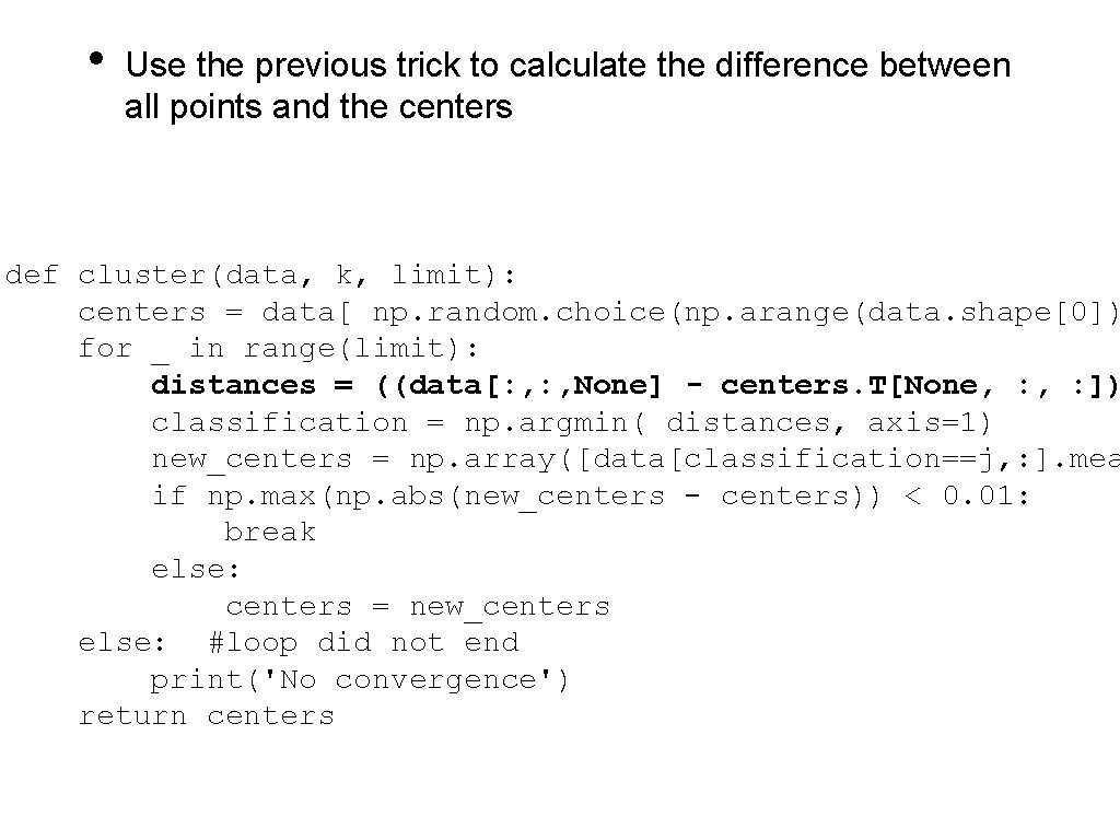
• Use the previous trick to calculate the difference between all points and the centers def cluster(data, k, limit): centers = data[ np. random. choice(np. arange(data. shape[0]) for _ in range(limit): distances = ((data[: , None] - centers. T[None, : ]) classification = np. argmin( distances, axis=1) new_centers = np. array([data[classification==j, : ]. mea if np. max(np. abs(new_centers - centers)) < 0. 01: break else: centers = new_centers else: #loop did not end print('No convergence') return centers

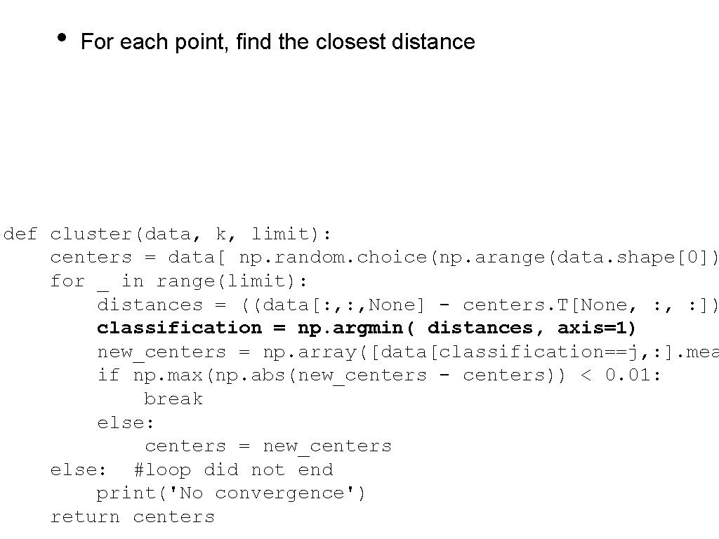
• For each point, find the closest distance def cluster(data, k, limit): centers = data[ np. random. choice(np. arange(data. shape[0]) for _ in range(limit): distances = ((data[: , None] - centers. T[None, : ]) classification = np. argmin( distances, axis=1) new_centers = np. array([data[classification==j, : ]. mea if np. max(np. abs(new_centers - centers)) < 0. 01: break else: centers = new_centers else: #loop did not end print('No convergence') return centers

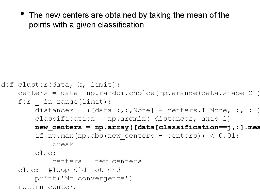
• The new centers are obtained by taking the mean of the points with a given classification def cluster(data, k, limit): centers = data[ np. random. choice(np. arange(data. shape[0]) for _ in range(limit): distances = ((data[: , None] - centers. T[None, : ]) classification = np. argmin( distances, axis=1) new_centers = np. array([data[classification==j, : ]. mea if np. max(np. abs(new_centers - centers)) < 0. 01: break else: centers = new_centers else: #loop did not end print('No convergence') return centers

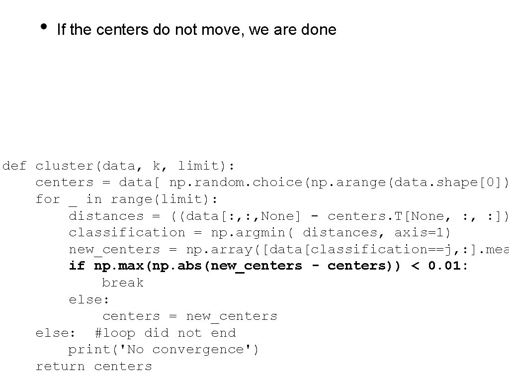
• If the centers do not move, we are done def cluster(data, k, limit): centers = data[ np. random. choice(np. arange(data. shape[0]) for _ in range(limit): distances = ((data[: , None] - centers. T[None, : ]) classification = np. argmin( distances, axis=1) new_centers = np. array([data[classification==j, : ]. mea if np. max(np. abs(new_centers - centers)) < 0. 01: break else: centers = new_centers else: #loop did not end print('No convergence') return centers

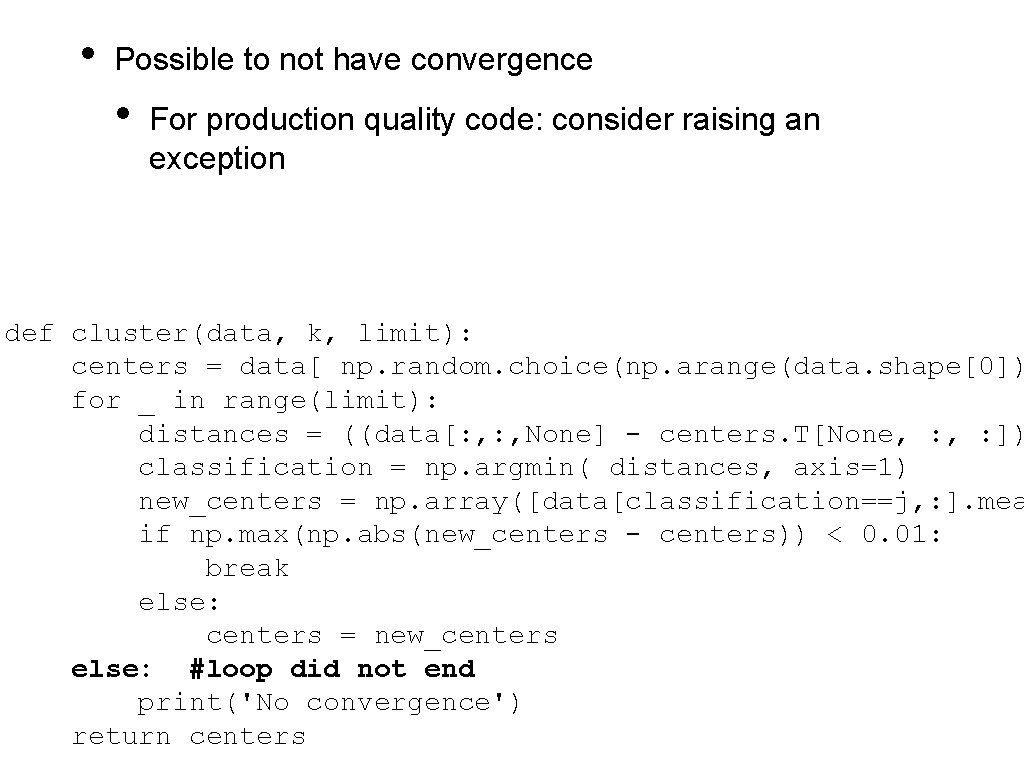
• Possible to not have convergence • For production quality code: consider raising an exception def cluster(data, k, limit): centers = data[ np. random. choice(np. arange(data. shape[0]) for _ in range(limit): distances = ((data[: , None] - centers. T[None, : ]) classification = np. argmin( distances, axis=1) new_centers = np. array([data[classification==j, : ]. mea if np. max(np. abs(new_centers - centers)) < 0. 01: break else: centers = new_centers else: #loop did not end print('No convergence') return centers

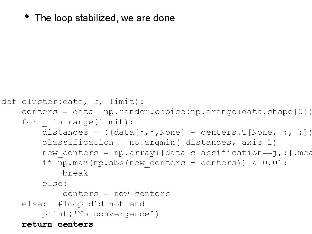
• The loop stabilized, we are done def cluster(data, k, limit): centers = data[ np. random. choice(np. arange(data. shape[0]) for _ in range(limit): distances = ((data[: , None] - centers. T[None, : ]) classification = np. argmin( distances, axis=1) new_centers = np. array([data[classification==j, : ]. mea if np. max(np. abs(new_centers - centers)) < 0. 01: break else: centers = new_centers else: #loop did not end print('No convergence') return centers

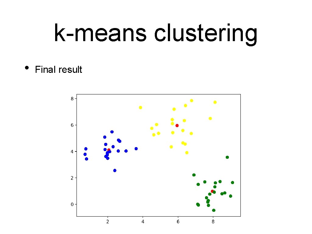
k-means clustering • Final result

k-means clustering • This worked because I used normalvariate to generate points around (2, 4), (8, 1), and (6, 6)

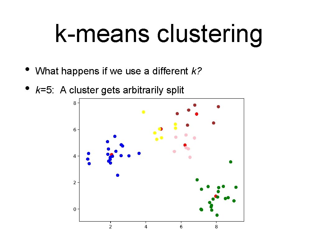
k-means clustering • • What happens if we use a different k? k=5: A cluster gets arbitrarily split

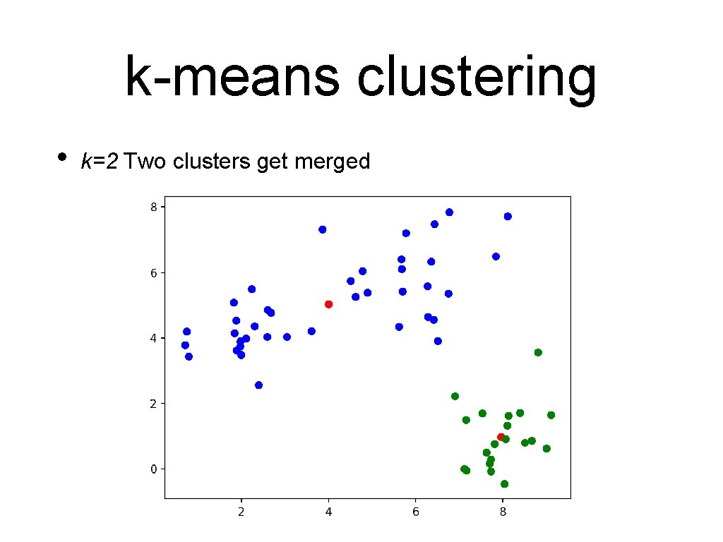
k-means clustering • k=2 Two clusters get merged

k-means clustering • Let's try this out on the Iris data set • • We only keep the measurements We can normalize data using the min-max method def normalize(array): maxs = np. max(array, axis = 0) mins = np. min(array, axis = 0) return (array-mins)/(maxs-mins)

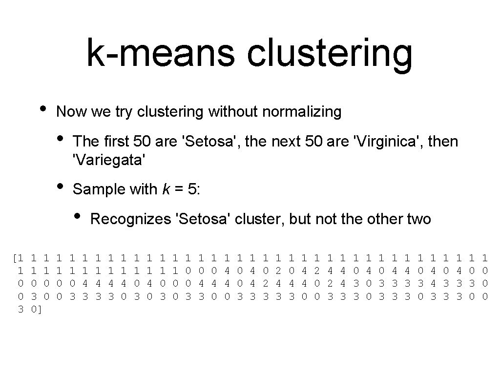
k-means clustering • Now we try clustering without normalizing • The first 50 are 'Setosa', the next 50 are 'Virginica', then 'Variegata' • Sample with k = 5: • [1 1 0 0 3 0 0] 1 1 0 0 1 1 0 3 Recognizes 'Setosa' cluster, but not the other two 1 1 4 3 1 1 4 0 1 1 0 3 1 1 0 0 3 1 0 4 0 1 4 4 0 1 0 0 3 1 4 4 3 1 0 2 3 1 2 4 3 1 0 4 3 1 4 4 0 1 2 0 0 1 4 2 3 1 4 4 3 1 0 3 3 1 4 0 0 1 0 3 3 1 4 3 3 1 0 3 0 1 4 4 3 1 0 3 3 1 4 3 3 1 0 3 0 1 0 0 0

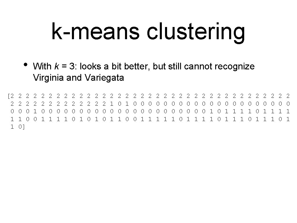
k-means clustering • [2 2 0 1 1 2 2 0 0 1 0 0] With k = 3: looks a bit better, but still cannot recognize Virginia and Variegata 2 2 1 0 2 2 0 1 2 2 0 0 2 2 0 1 2 2 0 0 2 1 0 1 2 0 0 1 2 1 0 0 2 0 0 1 2 0 0 1 2 0 0 0 2 0 0 1 2 0 1 1 2 0 0 0 2 0 1 1 2 0 1 0 2 0 0 1 2 0 1 0 2 0 1 1

k-means clustering • [1 1 0 0 0] Best results with k = 2: 1 1 0 0 1 1 0 0 1 1 0 0 0 1 0 0 0 1 0 1 1 0 0 0 1 0 0 0 1 0 0 0 1 0 0 0 1 0 0 0

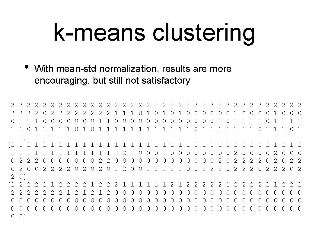
k-means clustering • [2 2 0 1 1 [1 1 0 0 2 [1 2 0 0 0 2 2 1 1 1 0 1] 1 1 2 2 2 0 0] 2 2 0 0 0] With mean-std normalization, results are more encouraging, but still not satisfactory 2 2 1 1 2 0 0 1 2 2 0 0 2 2 0 1 2 2 0 0 2 2 1 1 2 1 0 1 2 0 0 1 2 1 0 1 2 0 0 0 2 0 0 1 2 0 1 1 2 0 0 1 2 1 1 1 2 0 1 0 2 0 0 1 2 1 1 1 2 0 1 0 2 0 1 1 0 2 1 1 0 0 1 1 0 2 1 1 0 0 1 1 2 2 1 1 2 0 2 1 2 0 0 1 0 0 2 1 2 0 2 1 0 0 0 1 0 0 2 1 0 2 2 1 0 0 0 1 2 2 2 1 0 2 0 1 0 0 2 1 2 2 2 1 0 0 2 1 0 2 0 1 0 2 2 0 0 1 2 0 0 2 1 0 0 1 2 0 0 2 1 0 0 2 2 0 0 0 1 0 0 0 1 0 0 0 2 0 0 0 2 0 0 0 2 0 0 0 1 0 0 0

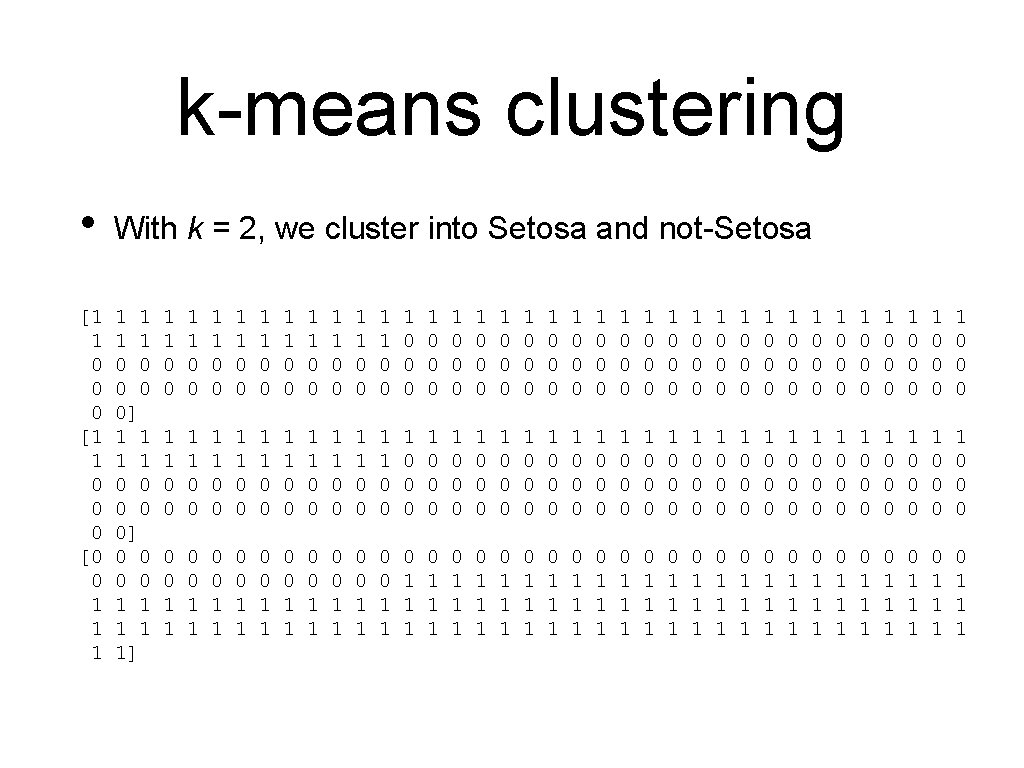
k-means clustering • With k = 2, we cluster into Setosa and not-Setosa [1 1 0 0 0 [0 0 1 1 1 1 0 0 0] 0 0 1 1 1] 1 1 0 0 1 1 0 0 1 1 0 0 1 1 0 0 1 1 0 0 1 0 0 0 1 0 0 0 1 0 0 0 1 0 0 0 1 0 0 0 1 0 0 0 1 0 0 0 1 0 0 0 1 0 0 0 1 0 0 0 1 0 0 0 1 0 0 0 0 0 1 1 0 0 1 1 0 0 1 1 1 0 1 1 1 0 1 1 1 0 1 1 1 0 1 1 1 0 1 1 1 0 1 1 1

k-means clustering • With k=4: still no separation [0 3 1 2 2 [2 2 0 0 0 [2 1 0 0 0 3 3 3 0 2 2 2 1 1] 2 2 0 0 0 1 0] 1 1 1 2 0 0 0] 3 0 2 1 0 3 1 2 3 0 1 2 0 0 1 2 3 3 1 1 3 0 1 2 0 3 1 1 3 0 2 2 3 3 2 1 2 0 2 1 1 0 1 1 2 0 2 1 2 0 1 1 1 3 1 1 2 0 1 2 2 0 1 1 1 0 2 2 2 3 1 2 2 0 1 2 1 0 1 1 2 0 2 2 2 3 1 2 1 0 1 2 2 0 0 2 2 1 3 2 2 1 1 2 2 1 3 2 2 1 1 2 2 0 3 2 2 0 0 2 0 1 3 2 0 1 0 2 1 1 0 2 0 0 0 2 1 1 3 2 0 1 3 2 1 1 3 2 0 1 0 2 1 1 1 2 1 1 3 2 1 1 0 2 0 0 0 2 1 1 0 2 0 3 0 2 1 0 0 2 1 3 1 2 1 1 3 2 0 3 3 2 1 0 0 2 1 3 1 2 1 0 0 1 2 0 0 2 1 0 0 3 1 0 0 2 2 0 0 1 1 0 0 1 2 0 0 2 1 0 0 2 2 0 0 1 0 0 0 3 0 0 0 2 0 1 0 2 1 0 0 2 0 0 0 2 1 0 0 2 0 1 0 0 0 2 0 0 0 1 0 0 0 2 0 0 0 3 0 0 0 1 0 0 0 2 0 0 0

k-means clustering • Morale: • With k-means clustering • • Definitely need to normalize data set Need to repeat method many times • Pick the one with the lowest sum of Euclidean distances

Decision Trees Thomas Schwarz, SJ

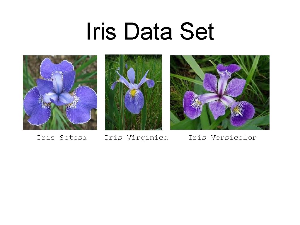
Decision Trees • One of many machine learning methods • • Used to learn categories Example: • The Iris Data Set • • Four measurements of flowers Learn how to predict species from measurement

Iris Data Set Iris Setosa Iris Virginica Iris Versicolor

Iris Data Set • Data in a. csv file • • Collected by Fisher One of the most famous datasets • Look it up on Kaggle or at UC Irvine Machine Learning Repository

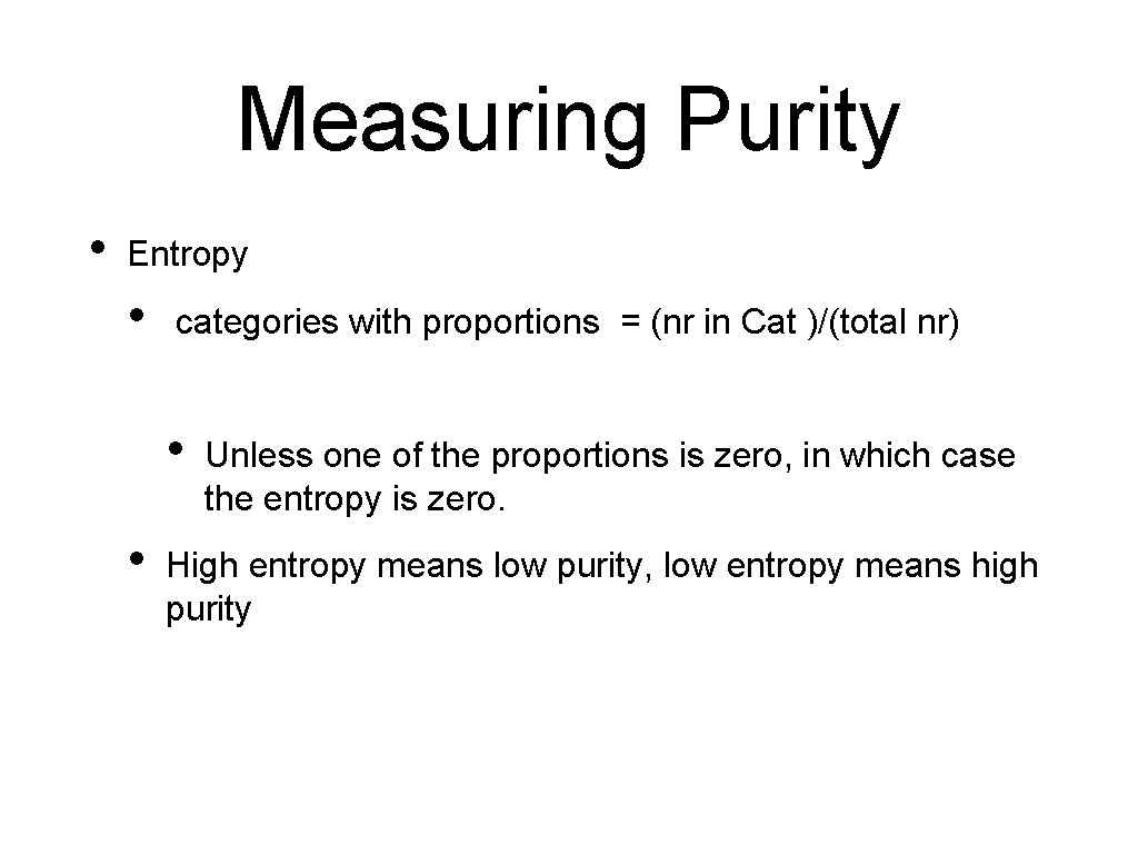
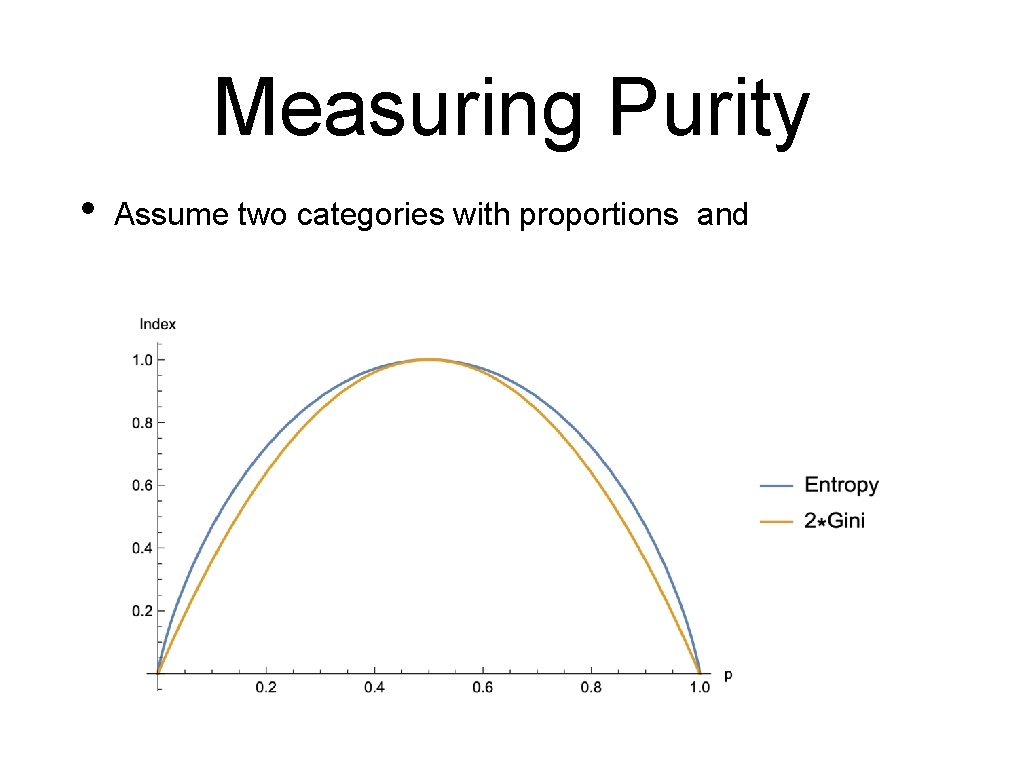
Measuring Purity • Entropy • categories with proportions = (nr in Cat )/(total nr) • • Unless one of the proportions is zero, in which case the entropy is zero. High entropy means low purity, low entropy means high purity

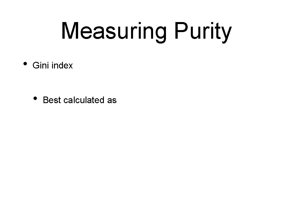
Measuring Purity • Gini index • Best calculated as

Measuring Purity • Assume two categories with proportions and

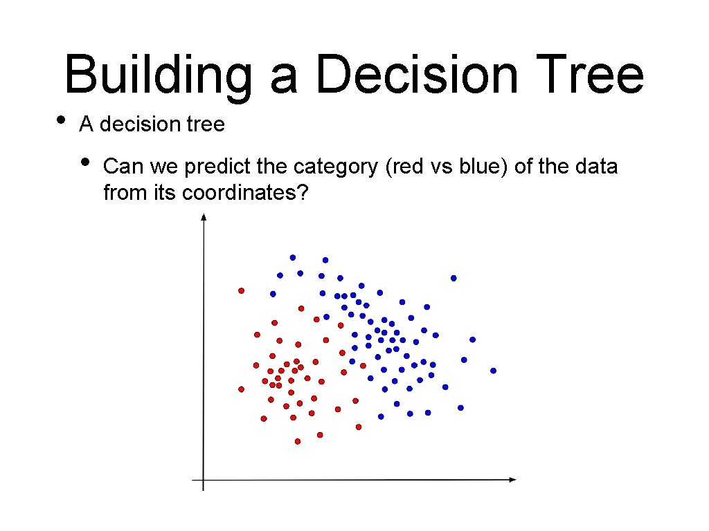
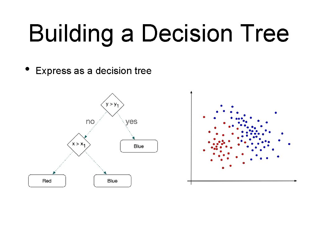
Building a Decision Tree • A decision tree • Can we predict the category (red vs blue) of the data from its coordinates?

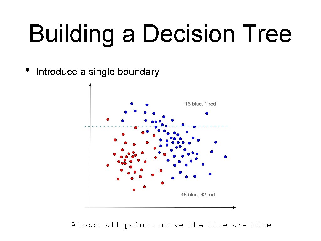
Building a Decision Tree • Introduce a single boundary Almost all points above the line are blue

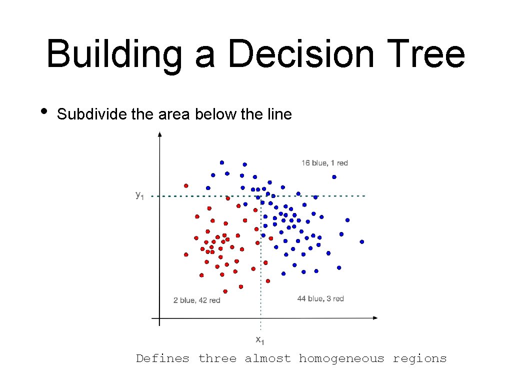
Building a Decision Tree • Subdivide the area below the line Defines three almost homogeneous regions

Building a Decision Tree • Express as a decision tree

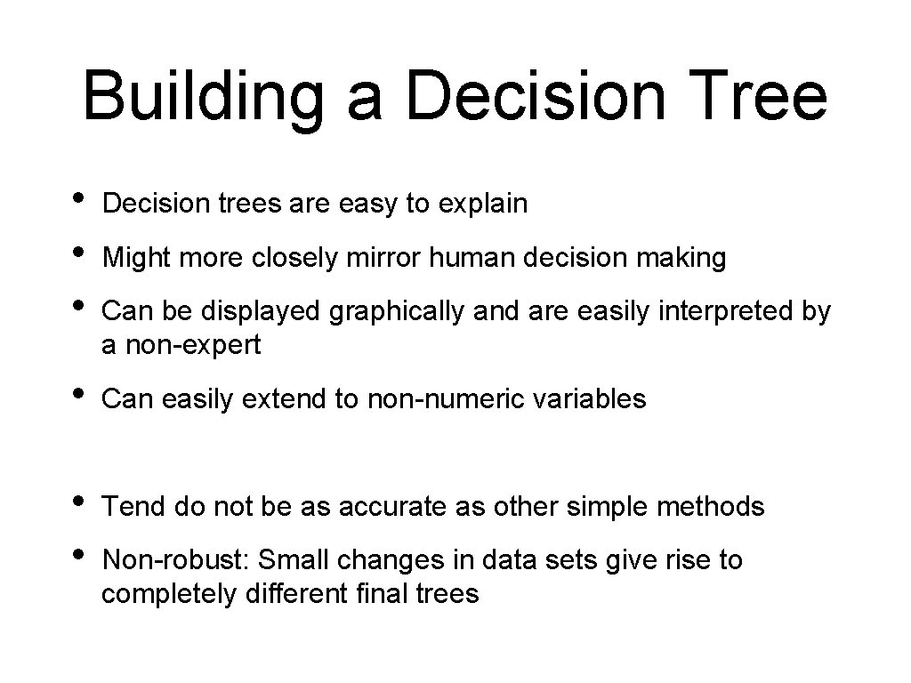
Building a Decision Tree • • • Decision trees are easy to explain • Can easily extend to non-numeric variables • • Tend do not be as accurate as other simple methods Might more closely mirror human decision making Can be displayed graphically and are easily interpreted by a non-expert Non-robust: Small changes in data sets give rise to completely different final trees

Building a Decision Tree • If a new point with coordinates (x, y) is considered • • Decision tree is not always correct even on the points used to develop it • • Use the decision tree to predict the color of the point But it is mostly right If new points behave like the old ones • Expect the rules to be mostly correct

Building a Decision Tree • How do we build decision trees • • Many algorithms were tried out and compared • Second rule: If decision rules are complex they are likely to not generalize First rule: Decisions should be simple, involving only one coordinate • E. g. : the lone red point in the upper region is probably an outlier and not indicative of general behavior

Building a Decision Tree • How do we build decision trees • Third rule: • Don't get carried away • Prune trees to avoid overfitting

Building a Decision Tree • Algorithm for decision trees: • Find a simple rule: • • Maximizes the information gain Continue sub-diving the regions • Stop when a region is homogeneous or almost homogeneous • Stop when a region becomes too small

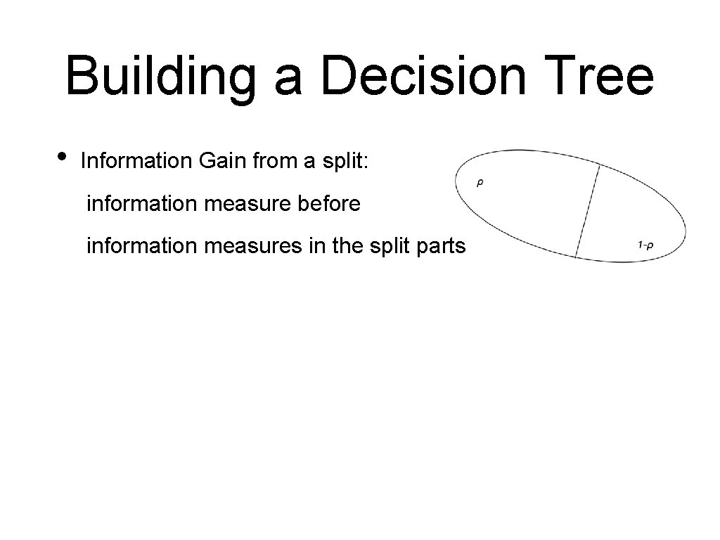
Building a Decision Tree • Information Gain from a split: information measure before information measures in the split parts

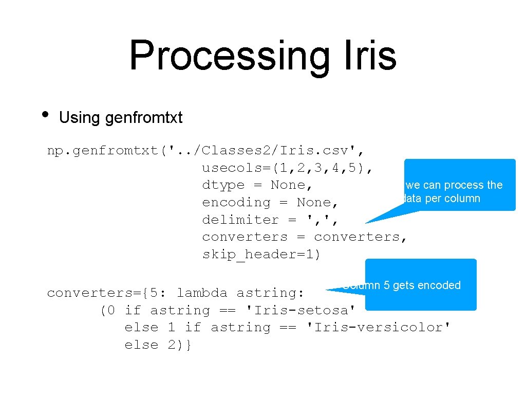
Processing Iris • We need to read in iris. csv • The last component is a string, which now needs an encoding (but we can pick the encoding to be None for the default) • We cannot use the default float type for the components

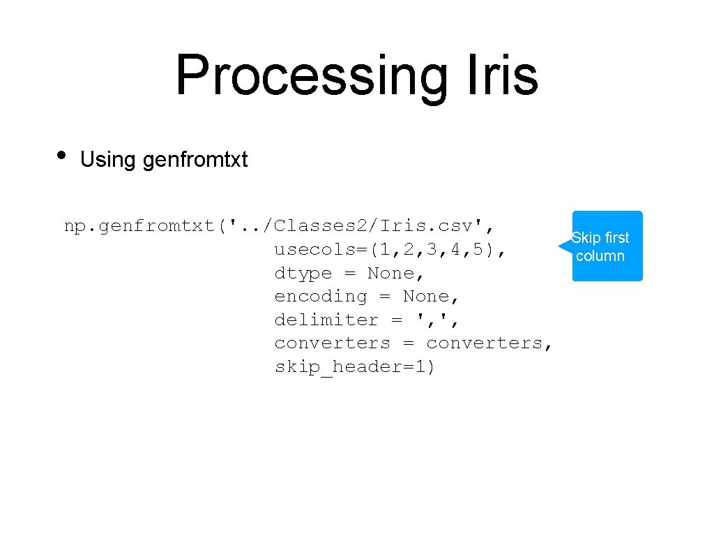
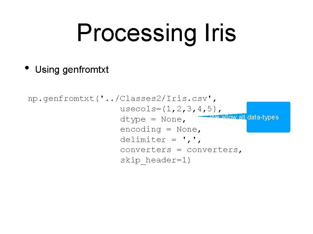
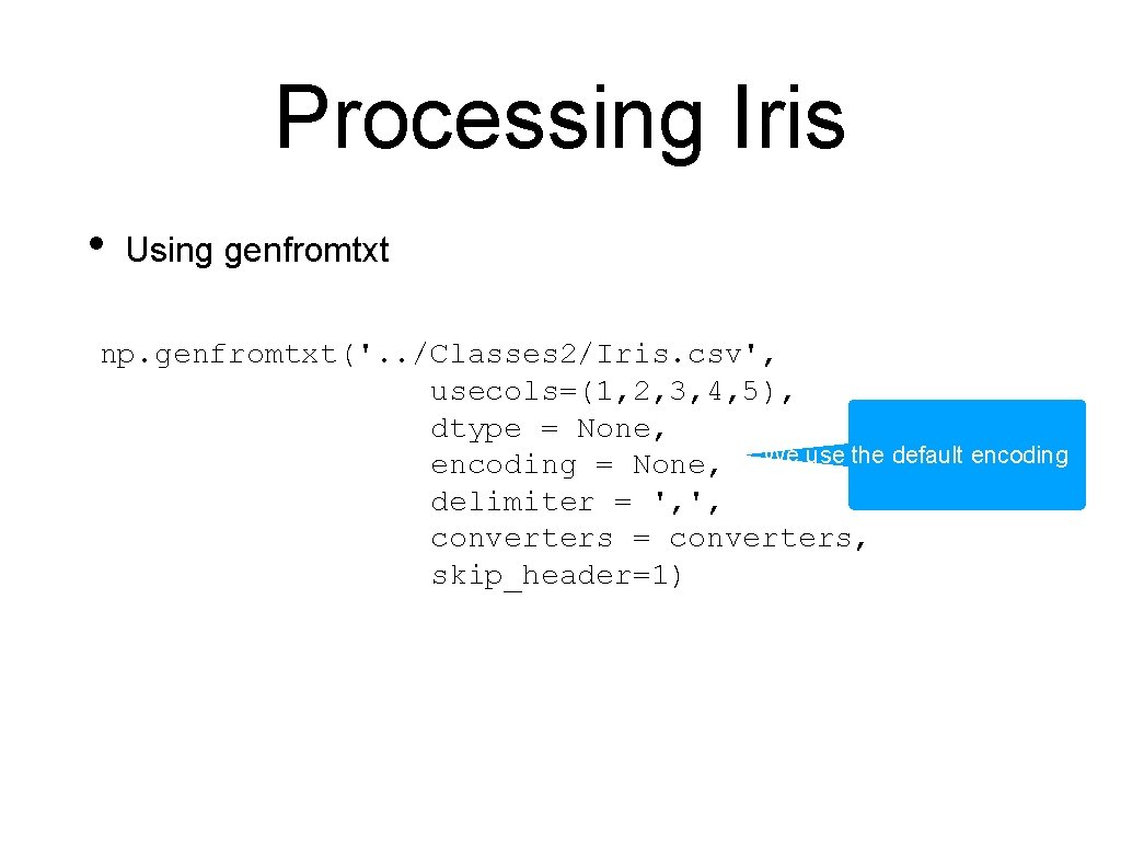
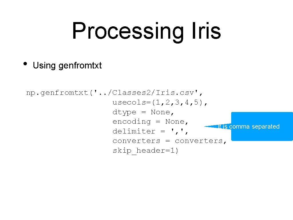
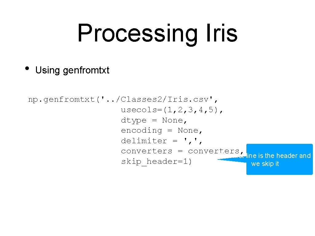
Processing Iris • Using genfromtxt np. genfromtxt('. . /Classes 2/Iris. csv', usecols=(1, 2, 3, 4, 5), dtype = None, encoding = None, delimiter = ', ', converters = converters, skip_header=1) Skip first column

Processing Iris • Using genfromtxt np. genfromtxt('. . /Classes 2/Iris. csv', usecols=(1, 2, 3, 4, 5), We allow all data-types dtype = None, encoding = None, delimiter = ', ', converters = converters, skip_header=1)

Processing Iris • Using genfromtxt np. genfromtxt('. . /Classes 2/Iris. csv', usecols=(1, 2, 3, 4, 5), dtype = None, encoding = None, We use the default encoding delimiter = ', ', converters = converters, skip_header=1)

Processing Iris • Using genfromtxt np. genfromtxt('. . /Classes 2/Iris. csv', usecols=(1, 2, 3, 4, 5), dtype = None, encoding = None, It is comma separated delimiter = ', ', converters = converters, skip_header=1)

Processing Iris • Using genfromtxt np. genfromtxt('. . /Classes 2/Iris. csv', usecols=(1, 2, 3, 4, 5), dtype = None, encoding = None, delimiter = ', ', converters = converters, The first line is the header and skip_header=1) we skip it

Processing Iris • Using genfromtxt np. genfromtxt('. . /Classes 2/Iris. csv', usecols=(1, 2, 3, 4, 5), Here we can process the dtype = None, data per column encoding = None, delimiter = ', ', converters = converters, skip_header=1) Column 5 gets encoded converters={5: lambda astring: (0 if astring == 'Iris-setosa' else 1 if astring == 'Iris-versicolor' else 2)}

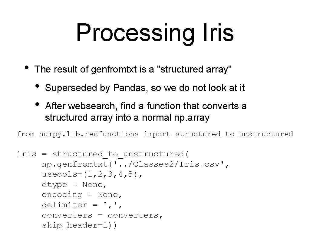
Processing Iris • The result of genfromtxt is a "structured array" • • Superseded by Pandas, so we do not look at it After websearch, find a function that converts a structured array into a normal np. array from numpy. lib. recfunctions import structured_to_unstructured iris = structured_to_unstructured( np. genfromtxt('. . /Classes 2/Iris. csv', usecols=(1, 2, 3, 4, 5), dtype = None, encoding = None, delimiter = ', ', converters = converters, skip_header=1))

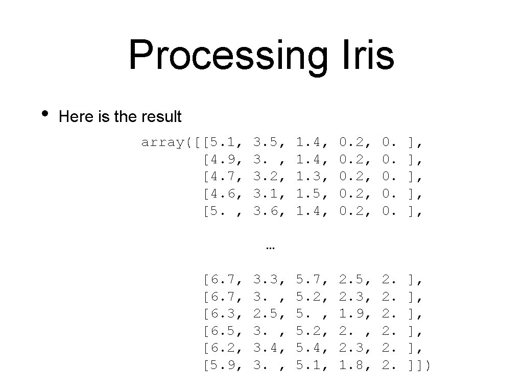
Processing Iris • Here is the result array([[5. 1, [4. 9, [4. 7, [4. 6, [5. , 3. 5, 3. 2, 3. 1, 3. 6, 1. 4, 1. 3, 1. 5, 1. 4, 0. 2, 0. 0. 0. ], ], ], 5. 7, 5. 2, 5. 4, 5. 1, 2. 5, 2. 3, 1. 9, 2. 3, 1. 8, 2. 2. 2. ], ], ], ]]) … [6. 7, [6. 3, [6. 5, [6. 2, [5. 9, 3. 3, 3. , 2. 5, 3. 4, 3. ,

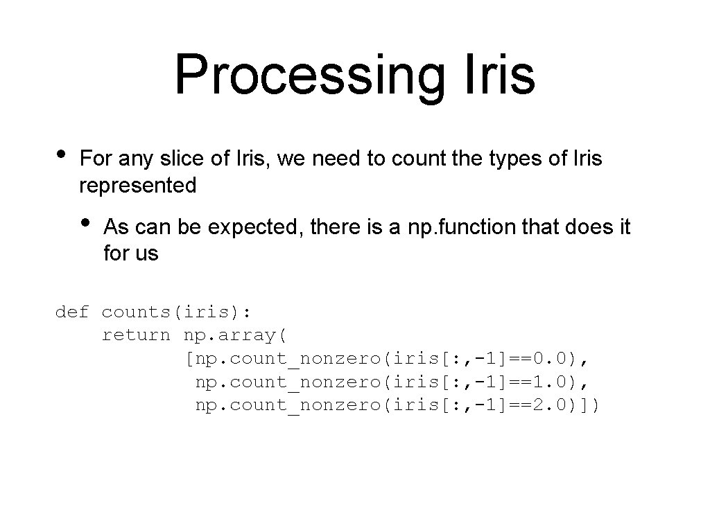
Processing Iris • For any slice of Iris, we need to count the types of Iris represented • As can be expected, there is a np. function that does it for us def counts(iris): return np. array( [np. count_nonzero(iris[: , -1]==0. 0), np. count_nonzero(iris[: , -1]==1. 0), np. count_nonzero(iris[: , -1]==2. 0)])

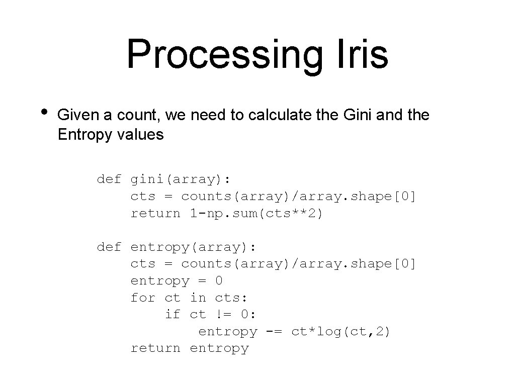
Processing Iris • Given a count, we need to calculate the Gini and the Entropy values def gini(array): cts = counts(array)/array. shape[0] return 1 -np. sum(cts**2) def entropy(array): cts = counts(array)/array. shape[0] entropy = 0 for ct in cts: if ct != 0: entropy -= ct*log(ct, 2) return entropy

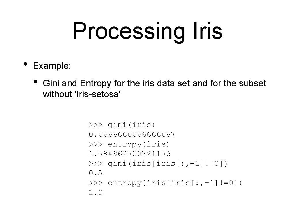
Processing Iris • Example: • Gini and Entropy for the iris data set and for the subset without 'Iris-setosa' >>> gini(iris) 0. 666666667 >>> entropy(iris) 1. 584962500721156 >>> gini(iris[: , -1]!=0]) 0. 5 >>> entropy(iris[: , -1]!=0]) 1. 0

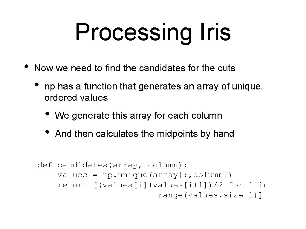
Processing Iris • Now we need to find the candidates for the cuts • np has a function that generates an array of unique, ordered values • • We generate this array for each column And then calculates the midpoints by hand def candidates(array, column): values = np. unique(array[: , column]) return [(values[i]+values[i+1])/2 for i in range(values. size-1)]

Processing Iris • Example: >>> np. unique(iris[: , 1]) array([2. , 2. 2, 2. 3, 2. 4, 2. 5, 2. 9, 3. 1, 3. 2, 3. 3, 3. 7, 3. 8, 3. 9, 4. 1, >>> candidates(iris, 1) [2. 1, 2. 25, 2. 3499999996, 2. 95, 3. 05, 3. 1500000004, 3. 3499999996, 3. 45, 3. 55, 3. 75, 3. 8499999996, 3. 95, 2. 6, 2. 7, 2. 8, 3. 4, 3. 5, 3. 6, 4. 2, 4. 4]) 2. 45, 2. 55, 2. 6500000 3. 25, 3. 6500000004, 4. 05, 4. 15, 4. 300000

Processing Iris • Remember how to split? >>> iris[: , 1]<2. 45] array([[4. 5, 2. 3, 1. 3, 0. 3, [5. 5, 2. 3, 4. , 1. 3, [4. 9, 2. 4, 3. 3, 1. , [5. , 2. , 3. 5, 1. , [6. , 2. 2, 4. , 1. , [6. 2, 2. 2, 4. 5, 1. 5, [5. 5, 2. 4, 3. 8, 1. 1, [5. 5, 2. 4, 3. 7, 1. , [6. 3, 2. 3, 4. 4, 1. 3, [5. , 2. 3, 3. 3, 1. , [6. , 2. 2, 5. , 1. 5, 0. 1. 1. 1. 2. ], ], ], ]])

Processing Iris • And how to count rows? >>> iris[: , 1]<2. 45]. shape (11, 5)

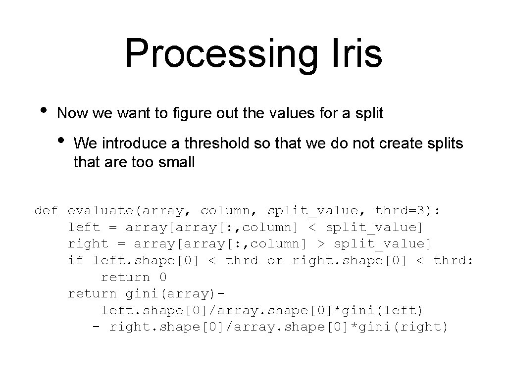
Processing Iris • Now we want to figure out the values for a split • We introduce a threshold so that we do not create splits that are too small def evaluate(array, column, split_value, thrd=3): left = array[: , column] < split_value] right = array[: , column] > split_value] if left. shape[0] < thrd or right. shape[0] < thrd: return 0 return gini(array)left. shape[0]/array. shape[0]*gini(left) - right. shape[0]/array. shape[0]*gini(right)

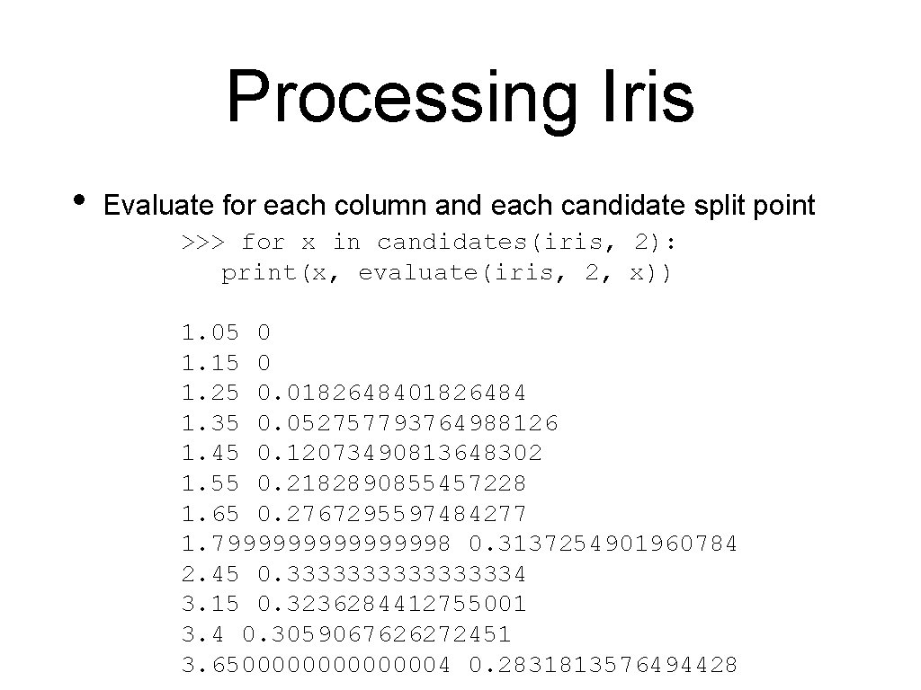
Processing Iris • Evaluate for each column and each candidate split point >>> for x in candidates(iris, 2): print(x, evaluate(iris, 2, x)) 1. 05 0 1. 15 0 1. 25 0. 01826484 1. 35 0. 052757793764988126 1. 45 0. 12073490813648302 1. 55 0. 2182890855457228 1. 65 0. 2767295597484277 1. 799999998 0. 3137254901960784 2. 45 0. 333333334 3. 15 0. 3236284412755001 3. 4 0. 3059067626272451 3. 6500000004 0. 2831813576494428

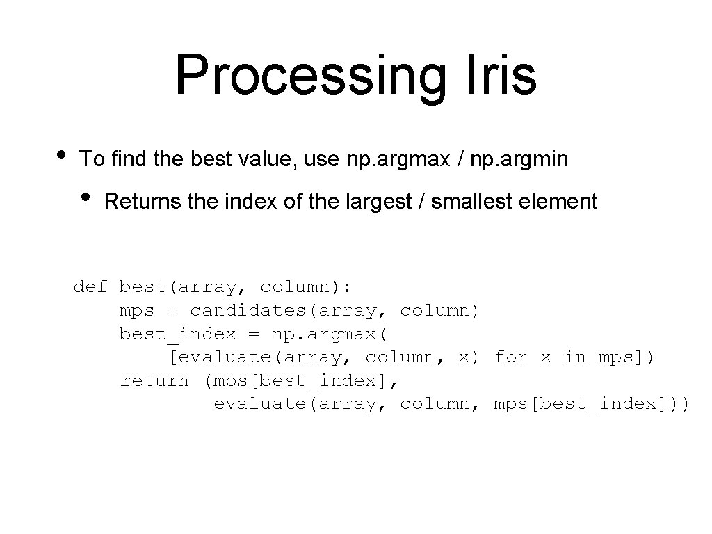
Processing Iris • To find the best value, use np. argmax / np. argmin • Returns the index of the largest / smallest element def best(array, column): mps = candidates(array, column) best_index = np. argmax( [evaluate(array, column, x) for x in mps]) return (mps[best_index], evaluate(array, column, mps[best_index]))

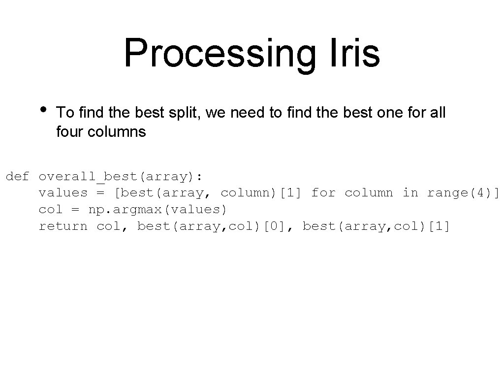
Processing Iris • To find the best split, we need to find the best one for all four columns def overall_best(array): values = [best(array, column)[1] for column in range(4)] col = np. argmax(values) return col, best(array, col)[0], best(array, col)[1]

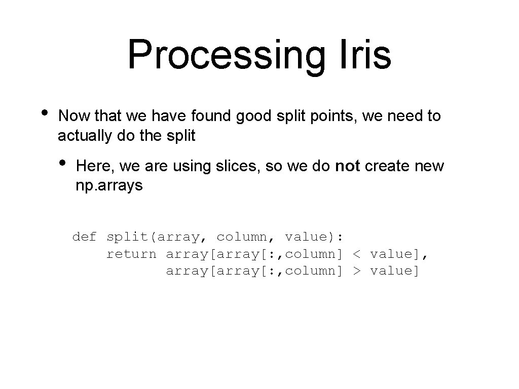
Processing Iris • Now that we have found good split points, we need to actually do the split • Here, we are using slices, so we do not create new np. arrays def split(array, column, value): return array[: , column] < value], array[: , column] > value]

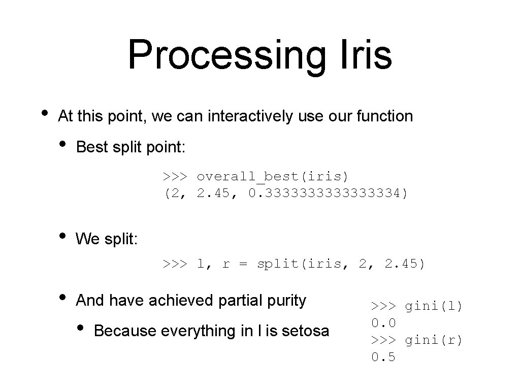
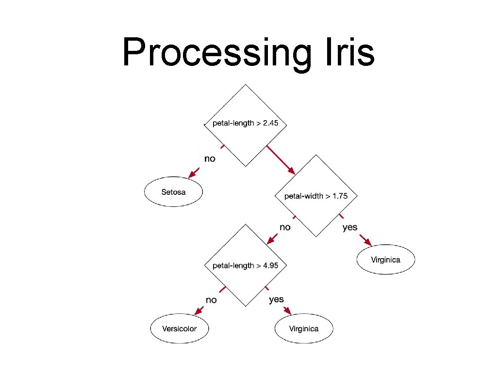
Processing Iris • At this point, we can interactively use our function • Best split point: >>> overall_best(iris) (2, 2. 45, 0. 333333334) • We split: >>> l, r = split(iris, 2, 2. 45) • And have achieved partial purity • Because everything in l is setosa >>> gini(l) 0. 0 >>> gini(r) 0. 5

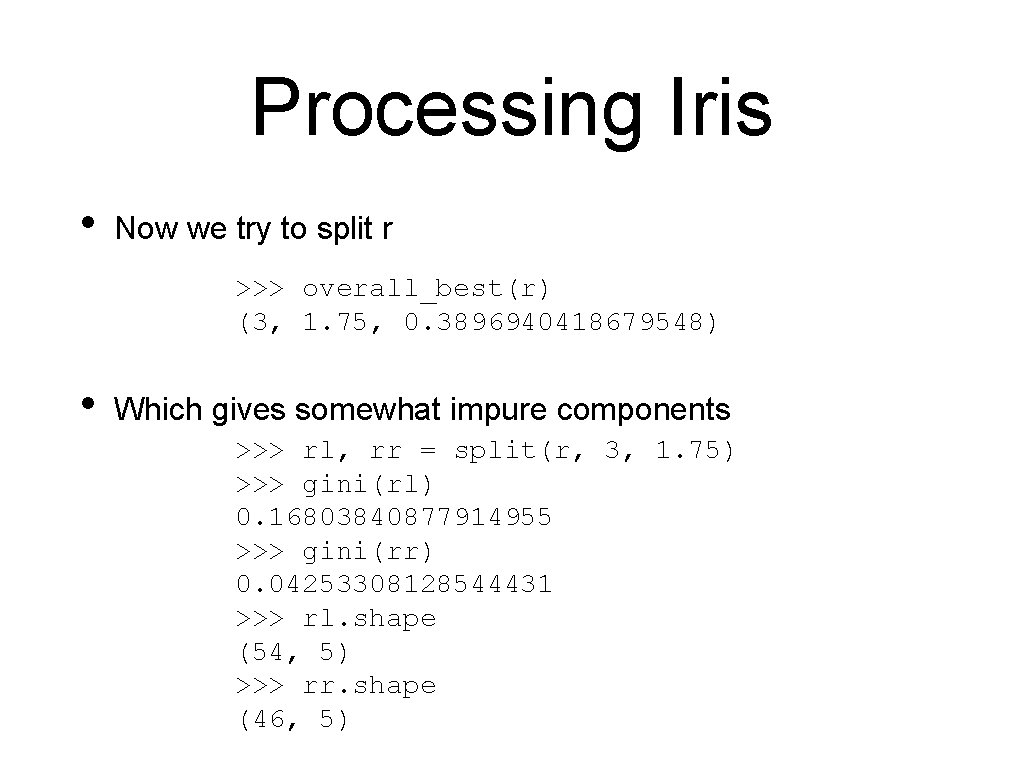
Processing Iris • Now we try to split r >>> overall_best(r) (3, 1. 75, 0. 3896940418679548) • Which gives somewhat impure components >>> rl, rr = split(r, 3, 1. 75) >>> gini(rl) 0. 16803840877914955 >>> gini(rr) 0. 04253308128544431 >>> rl. shape (54, 5) >>> rr. shape (46, 5)

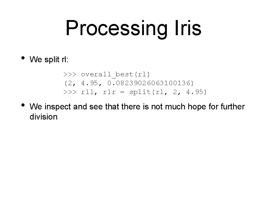
Processing Iris • We split rl: >>> overall_best(rl) (2, 4. 95, 0. 08239026063100136) >>> rll, rlr = split(rl, 2, 4. 95) • We inspect and see that there is not much hope for further division

Processing Iris • We look at rr and find it almost pure so we stop

Processing Iris

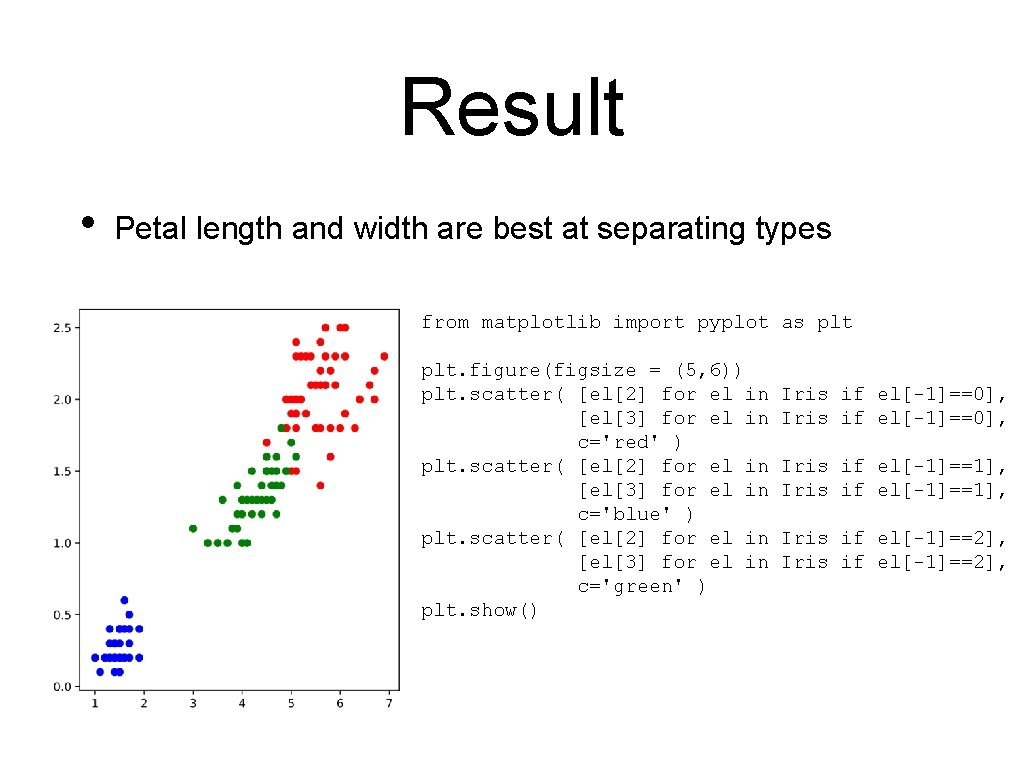
Result • Petal length and width are best at separating types from matplotlib import pyplot as plt. figure(figsize = (5, 6)) plt. scatter( [el[2] for el in [el[3] for el in c='red' ) plt. scatter( [el[2] for el in [el[3] for el in c='blue' ) plt. scatter( [el[2] for el in [el[3] for el in c='green' ) plt. show() Iris if el[-1]==0], Iris if el[-1]==1], Iris if el[-1]==2],

Testing • Let's implement the decision tree: def predict(element): if element[2] < 2. 45: return 1 else: if element[3] < 1. 75: if element[2] < 4. 95: return 2 else: return 0

Testing • And see how it works on the test data, taken randomly from the set • • One confused element or 1/36 error rate Total: • Four confused elements out of 150