import numpy as np import matplotlib pyplot as

import numpy as np import matplotlib. pyplot as plt import os for file in files: if file[0] == 'S': s. append(readfile(file)) def readfile (filename): if file[0] == 'T': data = [] t. append(readfile(file)) f = open (directory + '/' + filename, 'r') for line in f: s = np. array(s, dtype=float) data. append(line) t = np. array(t, dtype=float) f. close() return data i=0 directory = 'E: /python/data/oceans' files = os. listdir(directory) s = [] t = [] while i < s. shape[0]: plt. plot(s[i], t[i], 'o') print np. corrcoef(s[i], t[i])[0, 1] i=i+1 plt. show() 3

4

bands = 1 dt = gdal. GDT_Float 32 format = "GTiff" driver = gdal. Get. Driver. By. Name(format) raster = gdal. Open('E: /python/data/raster/B 4 B 5. tif') out. Data = driver. Create('E: /python/data/raster/output. tif', cols, rows, bands, dt ) red. Band = raster. Get. Raster. Band(1) out. Data. Set. Projection( projection ) red=red. Band. Read. As. Array(). astype(np. float 32) out. Data. Set. Geo. Transform( transform ) import gdal import matplotlib. pyplot as plt import numpy as np nir. Band = raster. Get. Raster. Band(2) nir=nir. Band. Read. As. Array(). astype(np. float 32) projection = raster. Get. Projection() transform = raster. Get. Geo. Transform() cols = raster. Raster. XSize rows = raster. Raster. YSize Add. Array = np. add(nir, red) Sub. Array = np. subtract(nir, red) np. seterr(divide='ignore') NDVIArray = np. divide(Sub. Array, Add. Array) out. Data. Get. Raster. Band( 1 ). Write. Array( NDVIArray ) plt. hist (nir) plt. hist (red) plt. show() 5

6

7

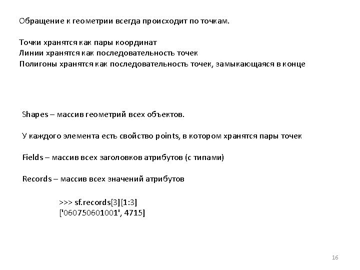
Пишем файлы тоже очень просто: Запишем точечный слой со своими точками import shapefile w = shapefile. Writer(shapefile. POINT) w. point(90. 3, 30) w. point(92, 40) w. point(-122. 4, 30) w. point(-90, 35. 1) w. field('FIRST_FLD') w. field('SECOND_FLD', 'C', '40') w. record('First', 'Point') w. record('Second', 'Point') w. record('Third', 'Point') w. record('Fourth', 'Point') w. save('E: /python/data/shp/point_test. shp') 17

Запишем слой со своим полигоном: import shapefile w = shapefile. Writer(shapefile. POINT) w = shapefile. Writer(shapefile. POLYGON) w. poly(parts=[[[1, 5], [5, 1], [3, 3], [1, 1]]]) w. field('FIRST_FLD', 'C', '40') w. field('SECOND_FLD', 'C', '40') w. record('First', 'Polygon') w. save('E: /python/data/shp/poly_test. shp') 18

Визуализировать shape-файл очень просто: import geovis. View. Shapefile("E: /python/data/shp/countries. shp") 21

Также очень просто сохранить shape-файл как изображение: geovis. Save. Shapefile. Image(" E: /python/data/shp/countries. shp ", savepath= «E: /output_picture. png") 22

Можно настраивать размеры карты, фон и прочее geovis. Set. Map. Dimensions(width=400, height=200) geovis. Set. Map. Background(geovis. Color("blue") newmap = geovis. New. Map() 24

Возможно раскрашивание по атрибутам polylayer = geovis. Layer('E: /python/data/shp/countries. shp', fillcolor=geovis. Color("red")) polylayer. Add. Classification(symboltype="fillcolor", valuefield="pop_est", symbolrange=[geovis. Color("#110000"), geovis. Color("#FF 0000")], classifytype="natural breaks", nrclasses=5) newmap = geovis. New. Map() newmap. Add. To. Map(polylayer) newmap. Save. Map('E: /map. png') 25

27

Спасибо за внимание! e. [email protected] ru ekazakov. info/students 28