MSCIT 5210 Knowledge Discovery and Data Mining Acknowledgement

MSCIT 5210: Knowledge Discovery and Data Mining Acknowledgement: Slides modified by Dr. Lei Chen based on the slides provided by Tan, Steinbach, Kumar And Jiawei Han, Micheline Kamber, and Jian Pei 1

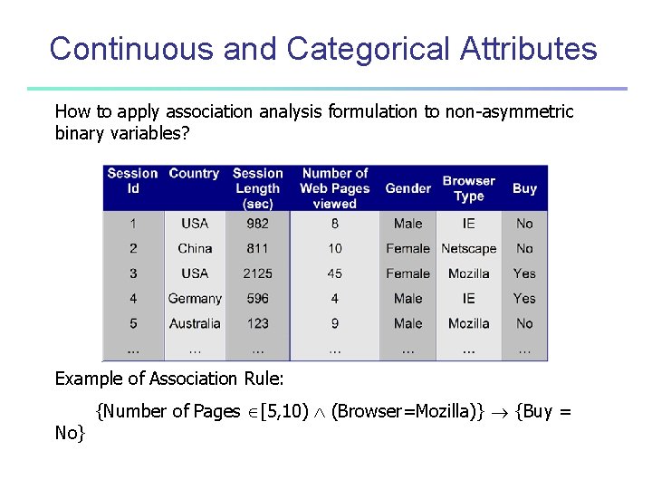
Continuous and Categorical Attributes How to apply association analysis formulation to non-asymmetric binary variables? Example of Association Rule: No} {Number of Pages [5, 10) (Browser=Mozilla)} {Buy =

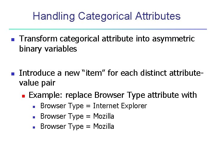
Handling Categorical Attributes n n Transform categorical attribute into asymmetric binary variables Introduce a new “item” for each distinct attributevalue pair n Example: replace Browser Type attribute with n n n Browser Type = Internet Explorer Browser Type = Mozilla

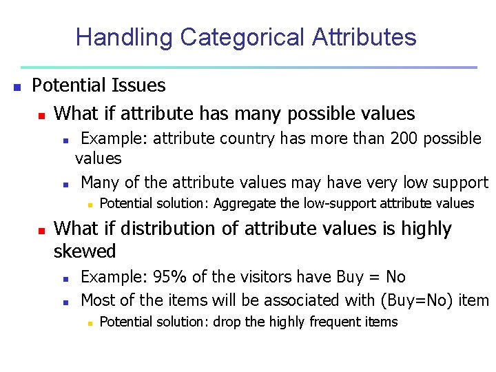
Handling Categorical Attributes n Potential Issues n What if attribute has many possible values n n Example: attribute country has more than 200 possible values Many of the attribute values may have very low support n n Potential solution: Aggregate the low-support attribute values What if distribution of attribute values is highly skewed n n Example: 95% of the visitors have Buy = No Most of the items will be associated with (Buy=No) item n Potential solution: drop the highly frequent items

Handling Continuous Attributes n n Different kinds of rules: n Age [21, 35) Salary [70 k, 120 k) Buy n Salary [70 k, 120 k) Buy Age: =28, =4 Different methods: n Discretization-based n Statistics-based n Non-discretization based n min. Apriori

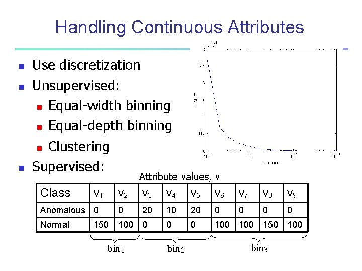
Handling Continuous Attributes n n n Use discretization Unsupervised: n Equal-width binning n Equal-depth binning n Clustering Supervised: Attribute values, v Class v 1 v 2 v 3 v 4 v 5 v 6 v 7 v 8 v 9 Anomalous 0 0 20 10 20 0 0 Normal 100 0 100 150 bin 1 bin 2 bin 3

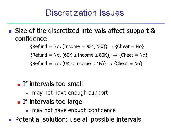
Discretization Issues n Size of the discretized intervals affect support & confidence {Refund = No, (Income = $51, 250)} {Cheat = No} {Refund = No, (60 K Income 80 K)} {Cheat = No} {Refund = No, (0 K Income 1 B)} {Cheat = No} n If intervals too small n n If intervals too large n n may not have enough support may not have enough confidence Potential solution: use all possible intervals

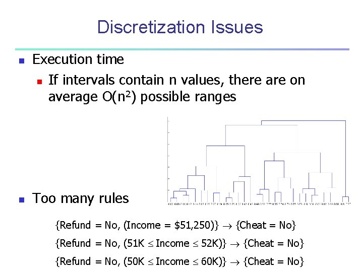
Discretization Issues n n Execution time n If intervals contain n values, there are on average O(n 2) possible ranges Too many rules {Refund = No, (Income = $51, 250)} {Cheat = No} {Refund = No, (51 K Income 52 K)} {Cheat = No} {Refund = No, (50 K Income 60 K)} {Cheat = No}

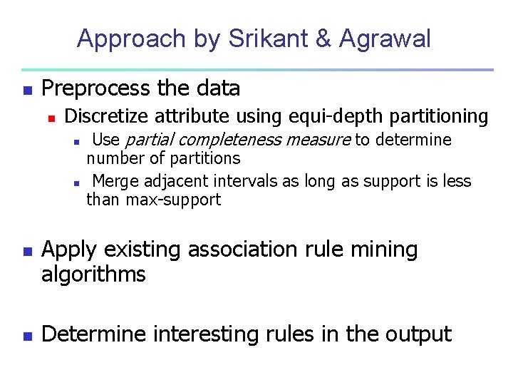
Approach by Srikant & Agrawal n Preprocess the data n Discretize attribute using equi-depth partitioning n n Use partial completeness measure to determine number of partitions Merge adjacent intervals as long as support is less than max-support Apply existing association rule mining algorithms Determine interesting rules in the output

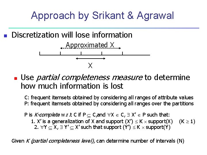
Approach by Srikant & Agrawal n Discretization will lose information Approximated X X n Use partial completeness measure to determine how much information is lost C: frequent itemsets obtained by considering all ranges of attribute values P: frequent itemsets obtained by considering all ranges over the partitions P is K-complete w. r. t C if P C, and X C, X’ P such that: 1. X’ is a generalization of X and support (X’) K support(X) 2. Y X, Y’ X’ such that support (Y’) K support(Y) (K 1) Given K (partial completeness level), can determine number of intervals (N)

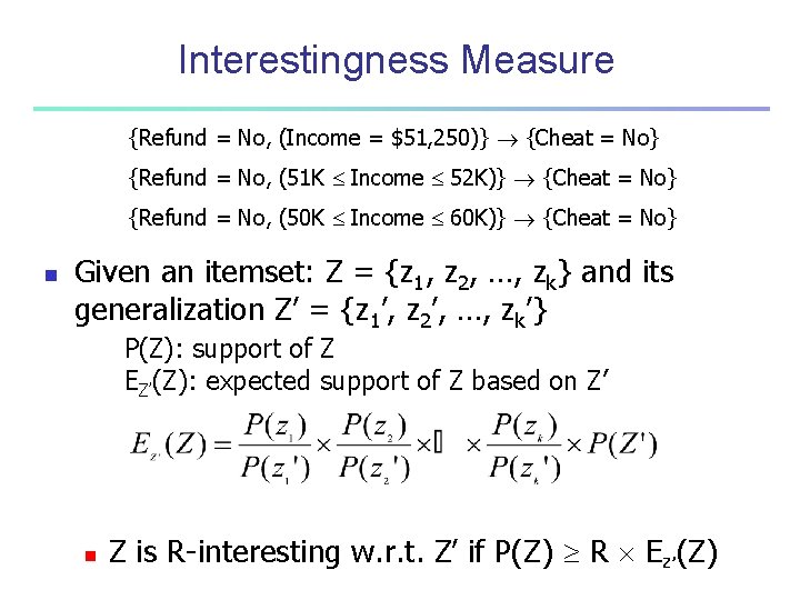
Interestingness Measure {Refund = No, (Income = $51, 250)} {Cheat = No} {Refund = No, (51 K Income 52 K)} {Cheat = No} {Refund = No, (50 K Income 60 K)} {Cheat = No} n Given an itemset: Z = {z 1, z 2, …, zk} and its generalization Z’ = {z 1’, z 2’, …, zk’} P(Z): support of Z EZ’(Z): expected support of Z based on Z’ n Z is R-interesting w. r. t. Z’ if P(Z) R EZ’(Z)

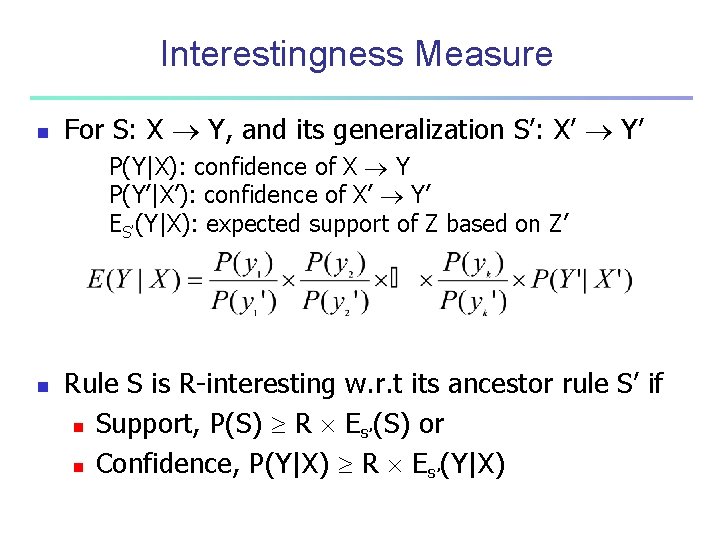
Interestingness Measure n For S: X Y, and its generalization S’: X’ Y’ P(Y|X): confidence of X Y P(Y’|X’): confidence of X’ Y’ ES’(Y|X): expected support of Z based on Z’ n Rule S is R-interesting w. r. t its ancestor rule S’ if n Support, P(S) R ES’(S) or n Confidence, P(Y|X) R ES’(Y|X)

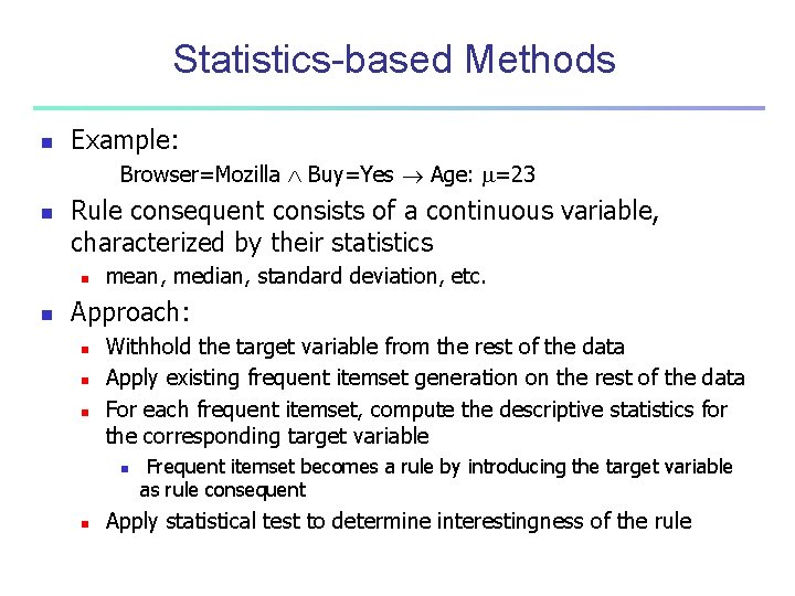
Statistics-based Methods n Example: Browser=Mozilla Buy=Yes Age: =23 n Rule consequent consists of a continuous variable, characterized by their statistics n n mean, median, standard deviation, etc. Approach: n n n Withhold the target variable from the rest of the data Apply existing frequent itemset generation on the rest of the data For each frequent itemset, compute the descriptive statistics for the corresponding target variable n n Frequent itemset becomes a rule by introducing the target variable as rule consequent Apply statistical test to determine interestingness of the rule

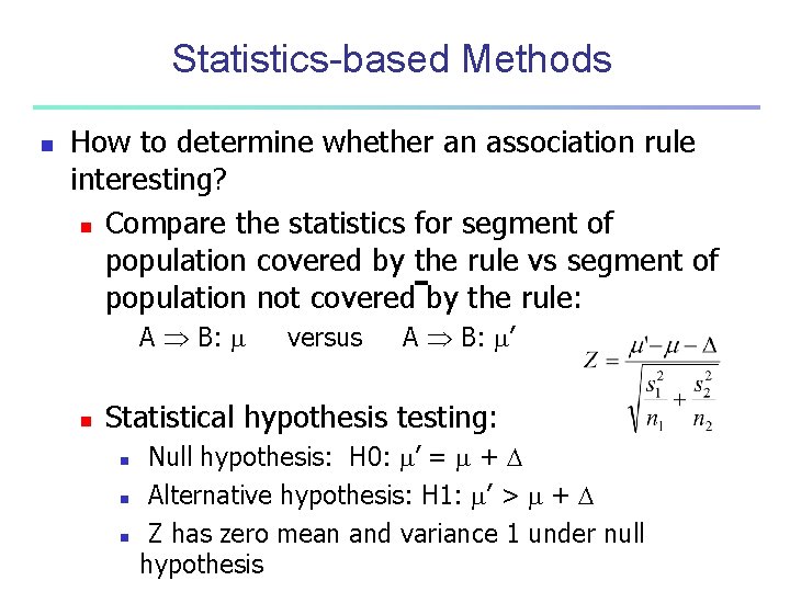
Statistics-based Methods n How to determine whether an association rule interesting? n Compare the statistics for segment of population covered by the rule vs segment of population not covered by the rule: A B: n versus A B: ’ Statistical hypothesis testing: n n n Null hypothesis: H 0: ’ = + Alternative hypothesis: H 1: ’ > + Z has zero mean and variance 1 under null hypothesis

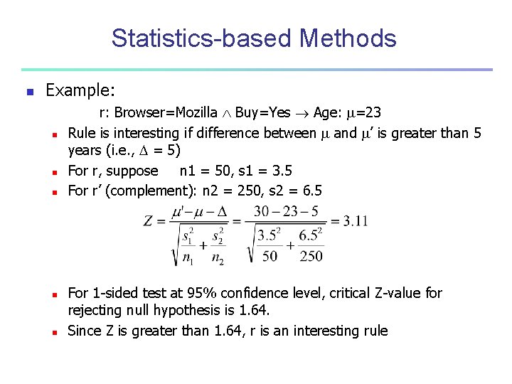
Statistics-based Methods n Example: n n n r: Browser=Mozilla Buy=Yes Age: =23 Rule is interesting if difference between and ’ is greater than 5 years (i. e. , = 5) For r, suppose n 1 = 50, s 1 = 3. 5 For r’ (complement): n 2 = 250, s 2 = 6. 5 For 1 -sided test at 95% confidence level, critical Z-value for rejecting null hypothesis is 1. 64. Since Z is greater than 1. 64, r is an interesting rule

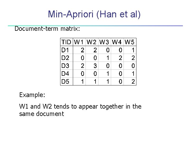
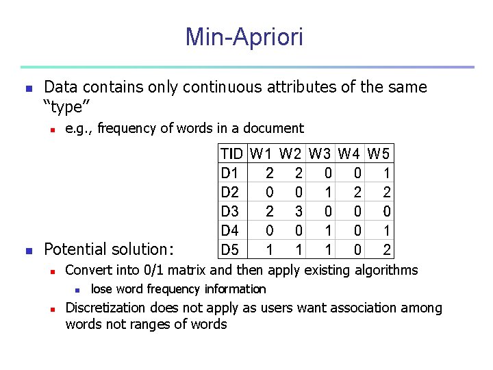
Min-Apriori (Han et al) Document-term matrix: Example: W 1 and W 2 tends to appear together in the same document

Min-Apriori n Data contains only continuous attributes of the same “type” n n e. g. , frequency of words in a document Potential solution: n Convert into 0/1 matrix and then apply existing algorithms n n lose word frequency information Discretization does not apply as users want association among words not ranges of words

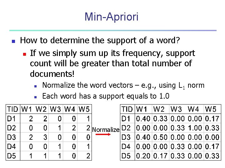
Min-Apriori n How to determine the support of a word? n If we simply sum up its frequency, support count will be greater than total number of documents! n n Normalize the word vectors – e. g. , using L 1 norm Each word has a support equals to 1. 0 Normalize

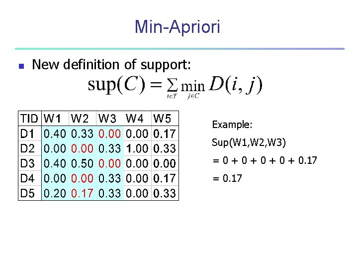
Min-Apriori n New definition of support: Example: Sup(W 1, W 2, W 3) = 0 + 0 + 0. 17 = 0. 17

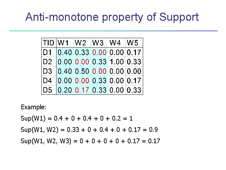
Anti-monotone property of Support Example: Sup(W 1) = 0. 4 + 0 + 0. 2 = 1 Sup(W 1, W 2) = 0. 33 + 0. 4 + 0. 17 = 0. 9 Sup(W 1, W 2, W 3) = 0 + 0 + 0. 17 = 0. 17

Multi-level Association Rules

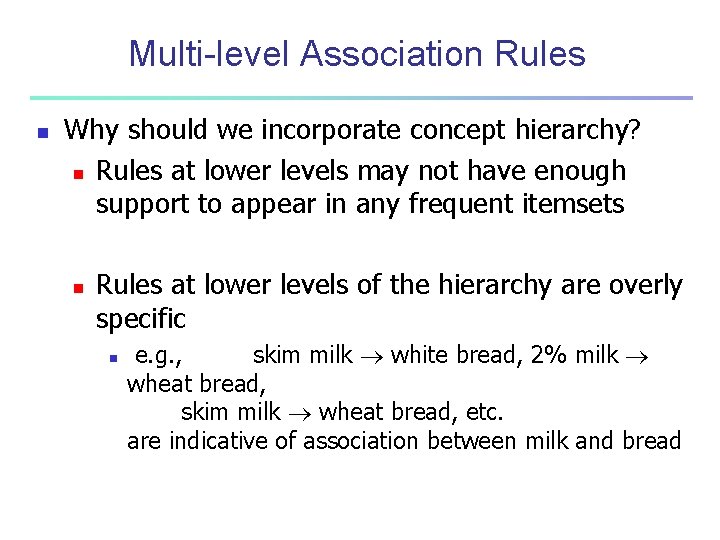
Multi-level Association Rules n Why should we incorporate concept hierarchy? n Rules at lower levels may not have enough support to appear in any frequent itemsets n Rules at lower levels of the hierarchy are overly specific n e. g. , skim milk white bread, 2% milk wheat bread, skim milk wheat bread, etc. are indicative of association between milk and bread

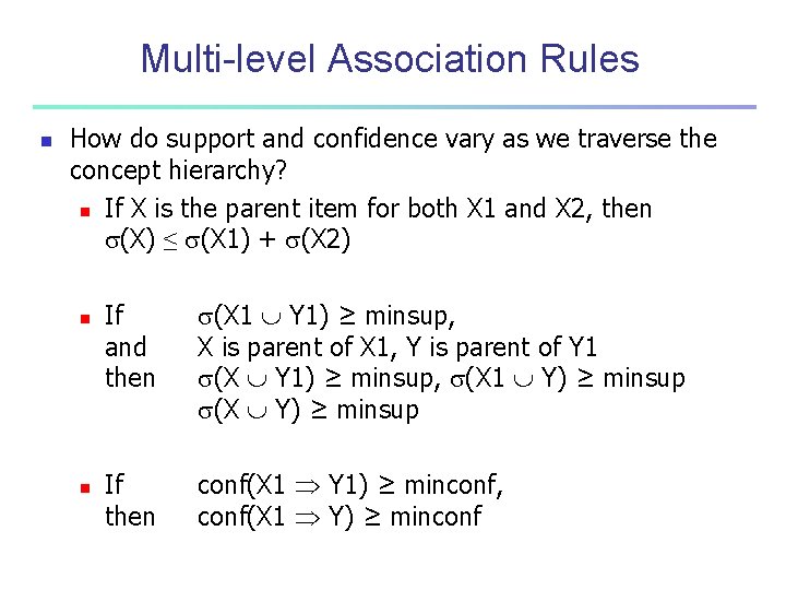
Multi-level Association Rules n How do support and confidence vary as we traverse the concept hierarchy? n If X is the parent item for both X 1 and X 2, then (X) ≤ (X 1) + (X 2) n n If and then (X 1 Y 1) ≥ minsup, X is parent of X 1, Y is parent of Y 1 (X Y 1) ≥ minsup, (X 1 Y) ≥ minsup (X Y) ≥ minsup If then conf(X 1 Y 1) ≥ minconf, conf(X 1 Y) ≥ minconf

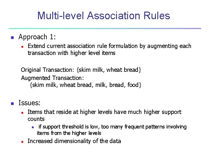
Multi-level Association Rules n Approach 1: n Extend current association rule formulation by augmenting each transaction with higher level items Original Transaction: {skim milk, wheat bread} Augmented Transaction: {skim milk, wheat bread, milk, bread, food} n Issues: n Items that reside at higher levels have much higher support counts n n if support threshold is low, too many frequent patterns involving items from the higher levels Increased dimensionality of the data

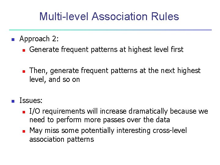
Multi-level Association Rules n Approach 2: n Generate frequent patterns at highest level first n n Then, generate frequent patterns at the next highest level, and so on Issues: n I/O requirements will increase dramatically because we need to perform more passes over the data n May miss some potentially interesting cross-level association patterns

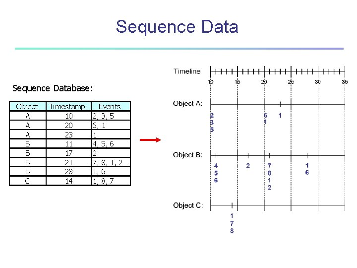
Sequence Database: Object A A A B B C Timestamp 10 20 23 11 17 21 28 14 Events 2, 3, 5 6, 1 1 4, 5, 6 2 7, 8, 1, 2 1, 6 1, 8, 7

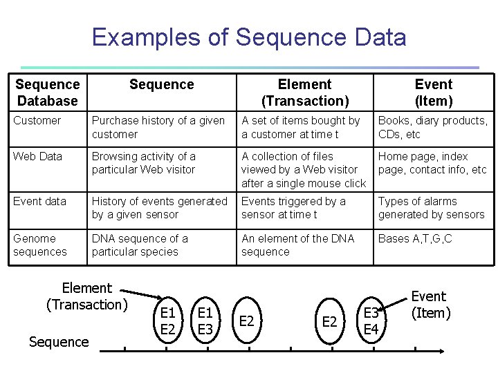
Examples of Sequence Database Sequence Element (Transaction) Event (Item) Customer Purchase history of a given customer A set of items bought by a customer at time t Books, diary products, CDs, etc Web Data Browsing activity of a particular Web visitor A collection of files viewed by a Web visitor after a single mouse click Home page, index page, contact info, etc Event data History of events generated by a given sensor Events triggered by a sensor at time t Types of alarms generated by sensors Genome sequences DNA sequence of a particular species An element of the DNA sequence Bases A, T, G, C Element (Transaction) Sequence E 1 E 2 E 1 E 3 E 2 E 3 E 4 Event (Item)

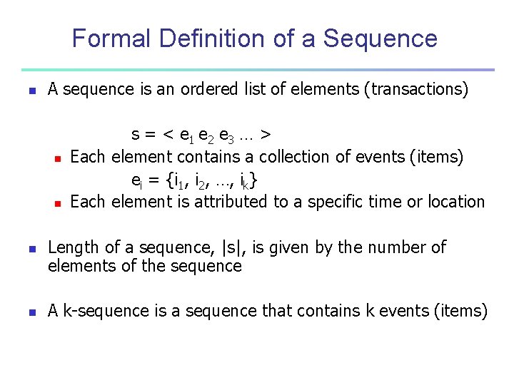
Formal Definition of a Sequence n A sequence is an ordered list of elements (transactions) n n s = < e 1 e 2 e 3 … > Each element contains a collection of events (items) ei = {i 1, i 2, …, ik} Each element is attributed to a specific time or location Length of a sequence, |s|, is given by the number of elements of the sequence A k-sequence is a sequence that contains k events (items)

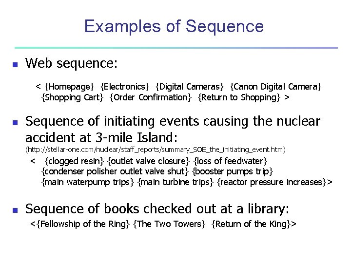
Examples of Sequence n Web sequence: < {Homepage} {Electronics} {Digital Cameras} {Canon Digital Camera} {Shopping Cart} {Order Confirmation} {Return to Shopping} > n Sequence of initiating events causing the nuclear accident at 3 -mile Island: (http: //stellar-one. com/nuclear/staff_reports/summary_SOE_the_initiating_event. htm) < {clogged resin} {outlet valve closure} {loss of feedwater} {condenser polisher outlet valve shut} {booster pumps trip} {main waterpump trips} {main turbine trips} {reactor pressure increases}> n Sequence of books checked out at a library: <{Fellowship of the Ring} {The Two Towers} {Return of the King}>

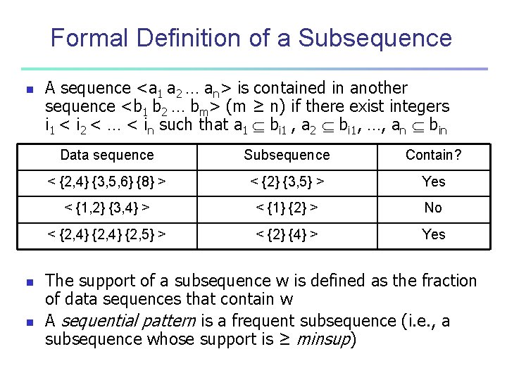
Formal Definition of a Subsequence n n n A sequence <a 1 a 2 … an> is contained in another sequence <b 1 b 2 … bm> (m ≥ n) if there exist integers i 1 < i 2 < … < in such that a 1 bi 1 , a 2 bi 1, …, an bin Data sequence Subsequence Contain? < {2, 4} {3, 5, 6} {8} > < {2} {3, 5} > Yes < {1, 2} {3, 4} > < {1} {2} > No < {2, 4} {2, 5} > < {2} {4} > Yes The support of a subsequence w is defined as the fraction of data sequences that contain w A sequential pattern is a frequent subsequence (i. e. , a subsequence whose support is ≥ minsup)

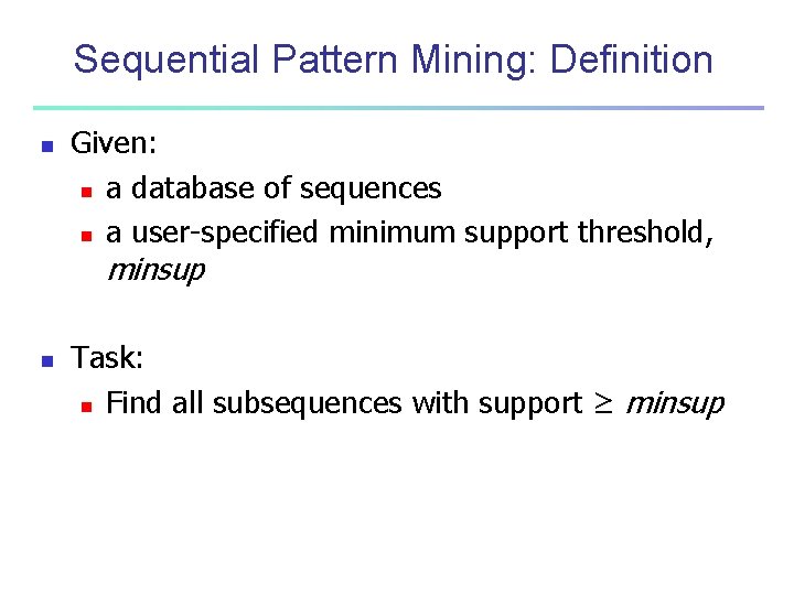
Sequential Pattern Mining: Definition n Given: n a database of sequences n a user-specified minimum support threshold, minsup n Task: n Find all subsequences with support ≥ minsup

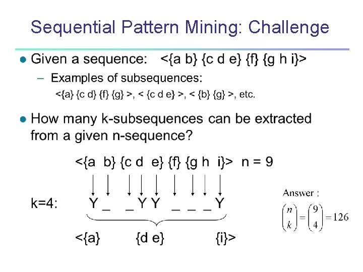
Sequential Pattern Mining: Challenge

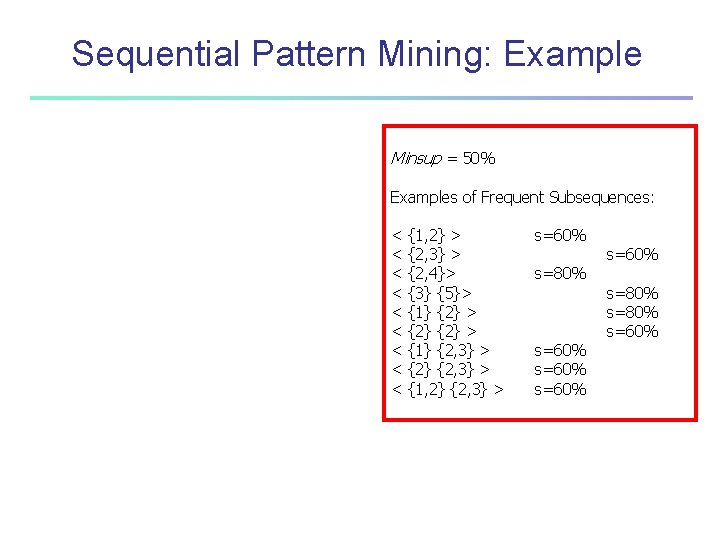
Sequential Pattern Mining: Example Minsup = 50% Examples of Frequent Subsequences: < < < < < {1, 2} > {2, 3} > {2, 4}> {3} {5}> {1} {2} > {1} {2, 3} > {2} {2, 3} > {1, 2} {2, 3} > s=60% s=80% s=60%

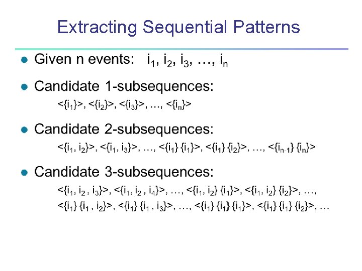
Extracting Sequential Patterns

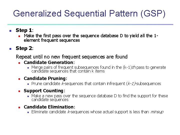
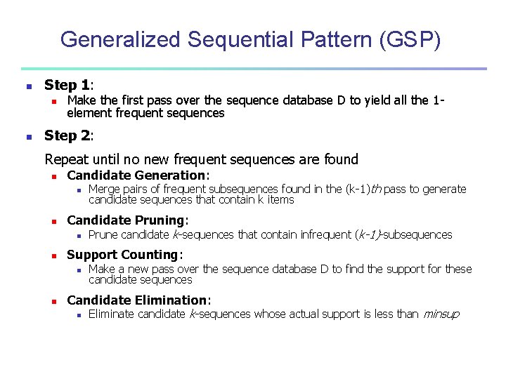
Generalized Sequential Pattern (GSP) n Step 1: n n Make the first pass over the sequence database D to yield all the 1 element frequent sequences Step 2: Repeat until no new frequent sequences are found n Candidate Generation: n n Candidate Pruning: n n Prune candidate k-sequences that contain infrequent (k-1)-subsequences Support Counting: n n Merge pairs of frequent subsequences found in the (k-1)th pass to generate candidate sequences that contain k items Make a new pass over the sequence database D to find the support for these candidate sequences Candidate Elimination: n Eliminate candidate k-sequences whose actual support is less than minsup

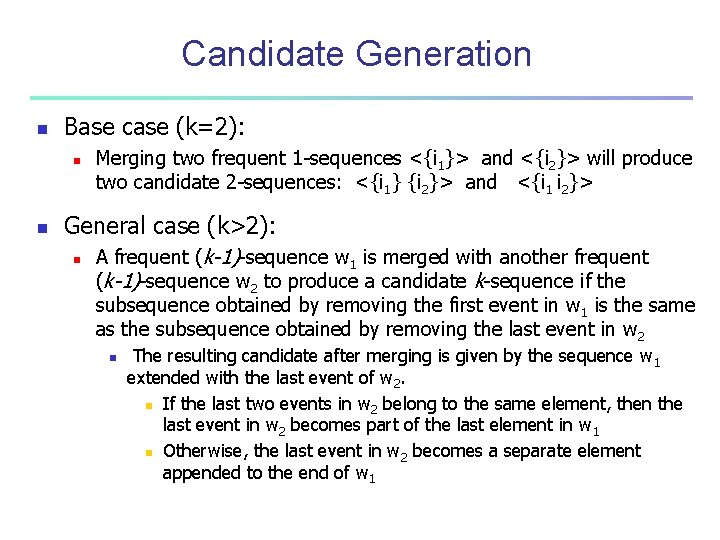
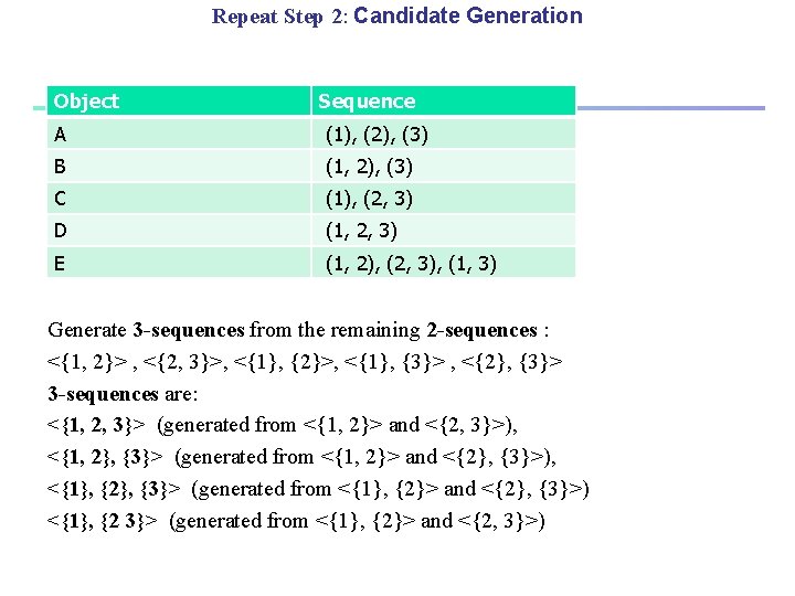
Candidate Generation n Base case (k=2): n n Merging two frequent 1 -sequences <{i 1}> and <{i 2}> will produce two candidate 2 -sequences: <{i 1} {i 2}> and <{i 1 i 2}> General case (k>2): n A frequent (k-1)-sequence w 1 is merged with another frequent (k-1)-sequence w 2 to produce a candidate k-sequence if the subsequence obtained by removing the first event in w 1 is the same as the subsequence obtained by removing the last event in w 2 n The resulting candidate after merging is given by the sequence w 1 extended with the last event of w 2. n If the last two events in w 2 belong to the same element, then the last event in w 2 becomes part of the last element in w 1 n Otherwise, the last event in w 2 becomes a separate element appended to the end of w 1

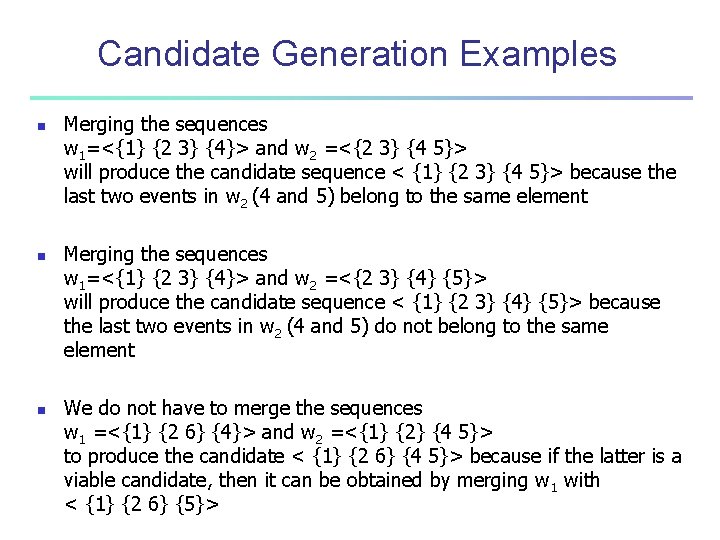
Candidate Generation Examples n n n Merging the sequences w 1=<{1} {2 3} {4}> and w 2 =<{2 3} {4 5}> will produce the candidate sequence < {1} {2 3} {4 5}> because the last two events in w 2 (4 and 5) belong to the same element Merging the sequences w 1=<{1} {2 3} {4}> and w 2 =<{2 3} {4} {5}> will produce the candidate sequence < {1} {2 3} {4} {5}> because the last two events in w 2 (4 and 5) do not belong to the same element We do not have to merge the sequences w 1 =<{1} {2 6} {4}> and w 2 =<{1} {2} {4 5}> to produce the candidate < {1} {2 6} {4 5}> because if the latter is a viable candidate, then it can be obtained by merging w 1 with < {1} {2 6} {5}>

Generalized Sequential Pattern (GSP) n Step 1: n n Make the first pass over the sequence database D to yield all the 1 element frequent sequences Step 2: Repeat until no new frequent sequences are found n Candidate Generation: n n Candidate Pruning: n n Prune candidate k-sequences that contain infrequent (k-1)-subsequences Support Counting: n n Merge pairs of frequent subsequences found in the (k-1)th pass to generate candidate sequences that contain k items Make a new pass over the sequence database D to find the support for these candidate sequences Candidate Elimination: n Eliminate candidate k-sequences whose actual support is less than minsup

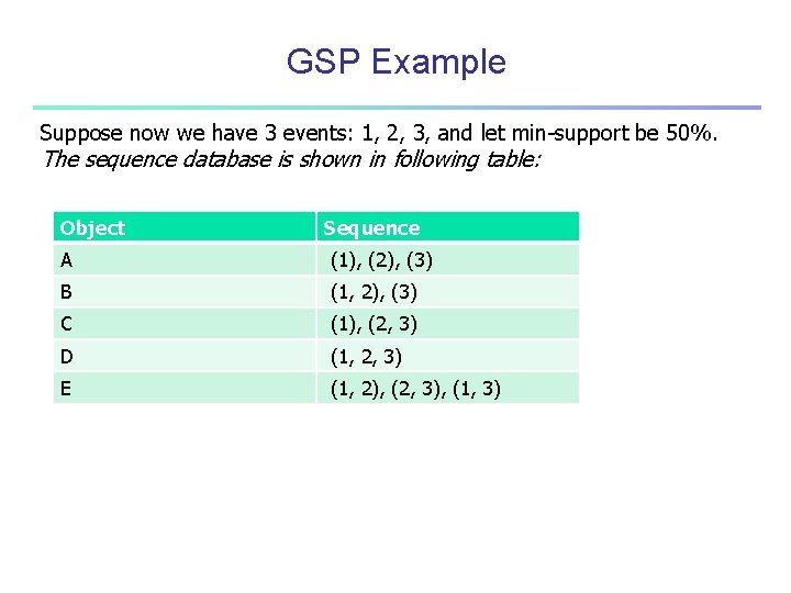
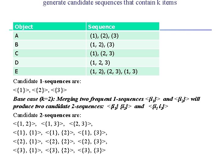
GSP Example Suppose now we have 3 events: 1, 2, 3, and let min-support be 50%. The sequence database is shown in following table: Object Sequence A (1), (2), (3) B (1, 2), (3) C (1), (2, 3) D (1, 2, 3) E (1, 2), (2, 3), (1, 3)

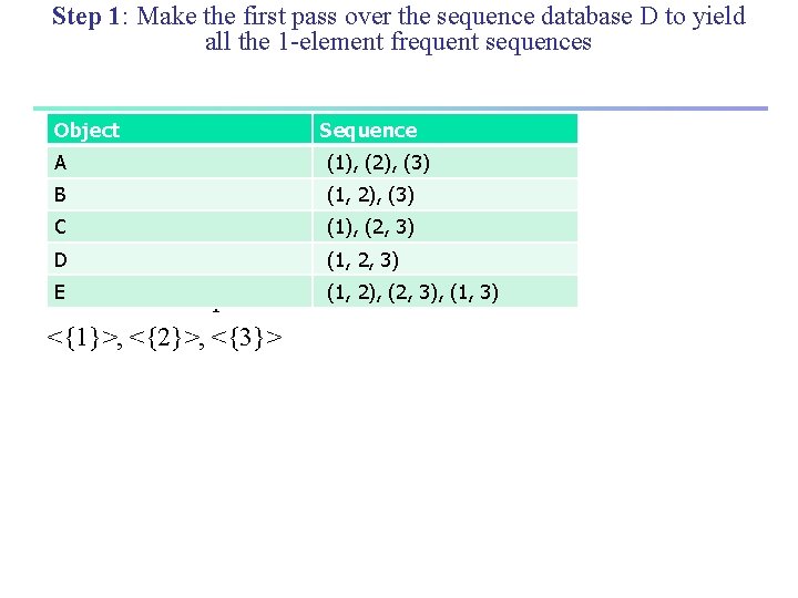
Step 1: Make the first pass over the sequence database D to yield all the 1 -element frequent sequences Object Sequence A (1), (2), (3) B (1, 2), (3) C (1), (2, 3) D (1, 2, 3) E Candidate 1 -sequences are: (1, 2), (2, 3), (1, 3) <{1}>, <{2}>, <{3}>

generate candidate sequences that contain k items Object Sequence A (1), (2), (3) B (1, 2), (3) C (1), (2, 3) D (1, 2, 3) E (1, 2), (2, 3), (1, 3) Candidate 1 -sequences are: <{1}>, <{2}>, <{3}> Base case (k=2): Merging two frequent 1 -sequences <{i 1}> and <{i 2}> will produce two candidate 2 -sequences: <{i 1} {i 2}> and <{i 1 i 2}> Candidate 2 -sequences are: <{1, 2}>, <{1, 3}>, <{2, 3}>, <{1}, {1}>, <{1}, {2}>, <{1}, {3}>, <{2}, {1}>, <{2}, {2}>, <{2}, {3}>, <{3}, {1}>, <{3}, {2}>, <{3}, {3}>

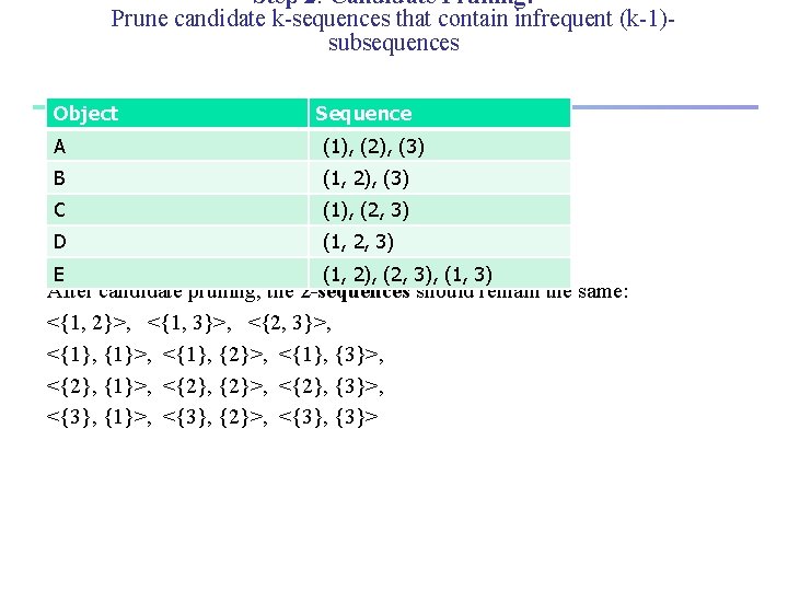
Step 2: Candidate Pruning: Prune candidate k-sequences that contain infrequent (k-1)subsequences Object Sequence A (1), (2), (3) B (1, 2), (3) C (1), (2, 3) D (1, 2, 3) E (1, 2), (2, 3), (1, 3) After candidate pruning, the 2 -sequences should remain the same: <{1, 2}>, <{1, 3}>, <{2, 3}>, <{1}, {1}>, <{1}, {2}>, <{1}, {3}>, <{2}, {1}>, <{2}, {2}>, <{2}, {3}>, <{3}, {1}>, <{3}, {2}>, <{3}, {3}>

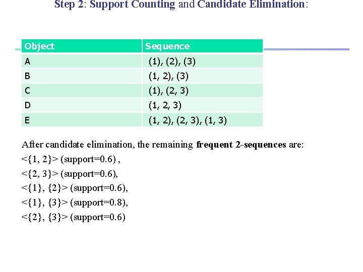
Step 2: Support Counting and Candidate Elimination: Object Sequence A (1), (2), (3) B (1, 2), (3) C (1), (2, 3) D (1, 2, 3) E (1, 2), (2, 3), (1, 3) After candidate elimination, the remaining frequent 2 -sequences are: <{1, 2}> (support=0. 6) , <{2, 3}> (support=0. 6), <{1}, {2}> (support=0. 6), <{1}, {3}> (support=0. 8), <{2}, {3}> (support=0. 6)

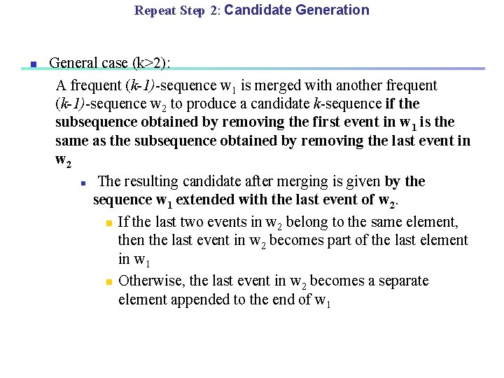
Repeat Step 2: Candidate Generation n General case (k>2): A frequent (k-1)-sequence w 1 is merged with another frequent (k-1)-sequence w 2 to produce a candidate k-sequence if the subsequence obtained by removing the first event in w 1 is the same as the subsequence obtained by removing the last event in w 2 n The resulting candidate after merging is given by the sequence w 1 extended with the last event of w 2. n If the last two events in w 2 belong to the same element, then the last event in w 2 becomes part of the last element in w 1 n Otherwise, the last event in w 2 becomes a separate element appended to the end of w 1

Repeat Step 2: Candidate Generation Object Sequence A (1), (2), (3) B (1, 2), (3) C (1), (2, 3) D (1, 2, 3) E (1, 2), (2, 3), (1, 3) Generate 3 -sequences from the remaining 2 -sequences : <{1, 2}> , <{2, 3}>, <{1}, {2}>, <{1}, {3}> , <{2}, {3}> 3 -sequences are: <{1, 2, 3}> (generated from <{1, 2}> and <{2, 3}>), <{1, 2}, {3}> (generated from <{1, 2}> and <{2}, {3}>), <{1}, {2}, {3}> (generated from <{1}, {2}> and <{2}, {3}>) <{1}, {2 3}> (generated from <{1}, {2}> and <{2, 3}>)

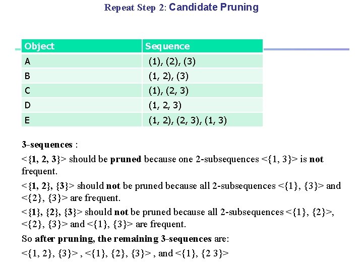
Repeat Step 2: Candidate Pruning Object Sequence A (1), (2), (3) B (1, 2), (3) C (1), (2, 3) D (1, 2, 3) E (1, 2), (2, 3), (1, 3) 3 -sequences : <{1, 2, 3}> should be pruned because one 2 -subsequences <{1, 3}> is not frequent. <{1, 2}, {3}> should not be pruned because all 2 -subsequences <{1}, {3}> and <{2}, {3}> are frequent. <{1}, {2}, {3}> should not be pruned because all 2 -subsequences <{1}, {2}>, <{2}, {3}> and <{1}, {3}> are frequent. So after pruning, the remaining 3 -sequences are: <{1, 2}, {3}> , <{1}, {2}, {3}> , and <{1}, {2 3}>

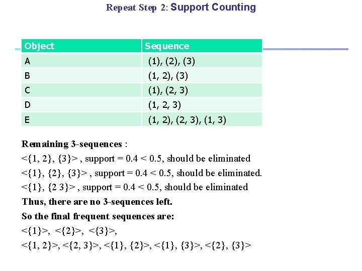
Repeat Step 2: Support Counting Object Sequence A (1), (2), (3) B (1, 2), (3) C (1), (2, 3) D (1, 2, 3) E (1, 2), (2, 3), (1, 3) Remaining 3 -sequences : <{1, 2}, {3}> , support = 0. 4 < 0. 5, should be eliminated <{1}, {2}, {3}> , support = 0. 4 < 0. 5, should be eliminated. <{1}, {2 3}> , support = 0. 4 < 0. 5, should be eliminated Thus, there are no 3 -sequences left. So the final frequent sequences are: <{1}>, <{2}>, <{3}>, <{1, 2}>, <{2, 3}>, <{1}, {2}>, <{1}, {3}>, <{2}, {3}>

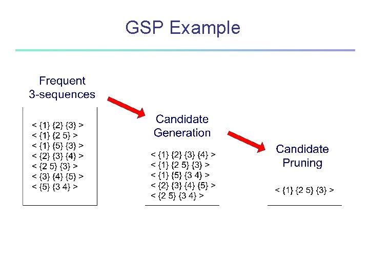
GSP Example

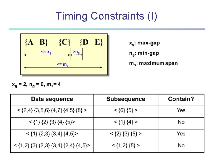
Timing Constraints (I)

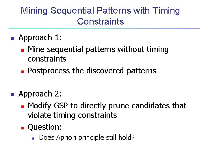
Mining Sequential Patterns with Timing Constraints n n Approach 1: n Mine sequential patterns without timing constraints n Postprocess the discovered patterns Approach 2: n Modify GSP to directly prune candidates that violate timing constraints n Question: n Does Apriori principle still hold?

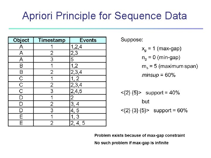
Apriori Principle for Sequence Data

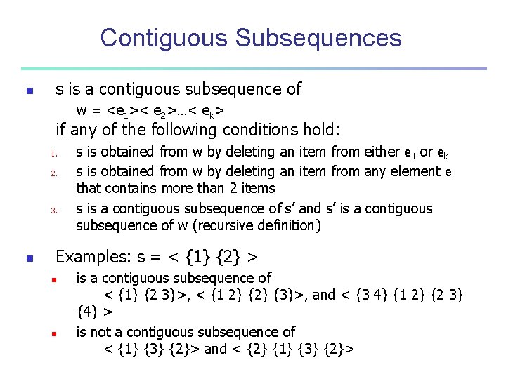
Contiguous Subsequences n s is a contiguous subsequence of w = <e 1>< e 2>…< ek> if any of the following conditions hold: 1. 2. 3. n s is obtained from w by deleting an item from either e 1 or ek s is obtained from w by deleting an item from any element ei that contains more than 2 items s is a contiguous subsequence of s’ and s’ is a contiguous subsequence of w (recursive definition) Examples: s = < {1} {2} > n n is a contiguous subsequence of < {1} {2 3}>, < {1 2} {3}>, and < {3 4} {1 2} {2 3} {4} > is not a contiguous subsequence of < {1} {3} {2}> and < {2} {1} {3} {2}>

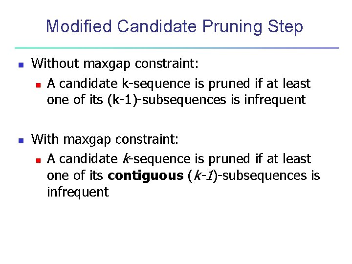
Modified Candidate Pruning Step n n Without maxgap constraint: n A candidate k-sequence is pruned if at least one of its (k-1)-subsequences is infrequent With maxgap constraint: n A candidate k-sequence is pruned if at least one of its contiguous (k-1)-subsequences is infrequent