Data Mining Data Mining DM Knowledge Discovery in

Data Mining

Data Mining (DM)/ Knowledge Discovery in Databases (KDD) “The nontrivial extraction of implicit, previously unknown, and potentially useful information from data” [Frawley et al, 1992]

Need for Data Mining u. Increased u. Remote ability to generate data sensors and satellites u. Bar codes for commercial products u. Computerization of businesses

Need for Data Mining u Increased u Media: ability to store data bigger magnetic disks, CD-ROMs u Better database management systems u Data warehousing technology

Need for Data Mining u Examples u Wal-Mart records 20, 000 transactions/day u Healthcare transactions yield multi-GB databases u Mobil Oil exploration storing 100 terabytes u Human Genome Project, multi-GBs and increasing u Astronomical object catalogs, terabytes of images u NASA EOS, 1 terabyte/day

Something for Everyone u u u Bell Atlantic MCI Land’s End Visa Bank of New York Fed. Ex

Market Analysis and Management u Customer profiling u. Data mining can tell you what types of customers buy what products (clustering or classification) or what products are often bought together (association rules). u Identifying customer requirements u Discover relationship between personal characteristics and probability of purchase u Discover correlations between purchases

Fraud Detection and Management u Applications: u Widely used in health care, retail, credit card services, telecommunications, etc. u Approach: u Use historical data to build models of fraudulent behavior and use data mining to help identify similar instances. u Examples: u Auto Insurance u Money Laundering u Medical Insurance

IBM Advertisement

DM step in KDD Process

Statistics Database AI Data Mining Hardware

Mining Association Rules

Mining Association Rules u u u Assocation rule mining: u Finding associations or correlations among a set of items or objects in transaction databases, relational databases, and data warehouses. Applications: u Basket data analysis, cross-marketing, catalog design, lossleader analysis, clustering, etc. Examples: u Rule form: “Body ® Head [support, confidence]”. u Buys=Diapers ® Buys=Beer [0. 5%, 60%] u Major=CS ^ Class=Data. Mining ® Grade=A [1%, 75%]

Rule Measures: Support and Confidence Customer buys both Customer buys beer Customer buys diaper u Find all the rules X & Y Z with minimum confidence and support u support, s, probability that a transaction contains {X, Y, Z} u confidence, c, conditional probability that a transaction having {X, Y} also contains Z. For minimum support 50%, minimum confidence 50%: A C (50%, 66. 6%) C A (50%, 100%)

Association Rule u u Given u Set of items I = {i 1, i 2, . . , im} u Set of transactions D u Each transaction T in D is a set of items An association rule is an implication u X and Y are itemsets, u Rule meets minimum confidence c (c% of transactions in D which contain X contain Y) u A minimum support s is also met c X ÈY / X s X ÈY / D

Mining Strong Association Rules in Transaction DBs u Measurement of rule strength in a transaction DB. A ® B [support, confidence] support = Prob(A È B) = #_of_trans_containing_all_the_items_in confidence = Prob(B|A) u u AÈB total_#_of_trans = #_of_trans_that_contain_both A and B #_of_trans_containing A We are often interested in only strong associations, i. e. support ³ min_sup and confidence ³ min_conf. Examples. milk ® bread [5%, 60%]. tire Ù auto_accessories ® auto_services [2%, 80%].

Methods for Mining Associations u Apriori u Partition Technique: u Sampling technique u Anti-Skew u Multi-level or generalized association u Constraint-based or query-based association

Apriori (Levelwise) u Scan database multiple times u For ith scan, find all large itemsets of size i with min support u Use the large itemsets from scan i as input to scan i+1 u Create candidates, subsets of size i+1 which contain only large itemsets as subsets u Notation: Large k-itemset, Lk Set of candidate large itemsets of size k, Ck u Note: If {A, B} is not a large itemset, then no superset of it can be either.

Mining Association Rules -- Example Min. support 50% Min. confidence 50% For rule A C: support = support({A, C}) = 50% confidence = support({A, C})/support({A}) = 66. 6% Apriori principle: Any subset of a frequent itemset must be frequent.

Minsup = 0. 25, Minconf = 0. 5 L 1 = {(A, 3), (B, 2), (C, 2), (D, 1), (E, 1), (F, 1)} C 2 = {(A, B), (A, C), (A, D), (A, E), (A, F), (B, C), . . , (E, F)} L 2 = {(A, B, 1), (A, C, 2), (A, D, 1), (B, C, 1), (B, F, 1), (E, F, 1)} (B, E, C 3 = {(A, B, C), (A, B, D), (A, C, D), (B, C, E), (B, C, F), (B, E, F)} L 3 = {(A, B, C, 1), (B, E, F, 1)} C 4 = {}, L 4 = {}, End of program Possible Rules A=>B (c=. 33, s=1), B=>A (c=. 5, s=1), A=>C (c=. 67, s=2), C=>A (c=1. 0, s=2) A=>D (c=. 33, s=1), D=>A (c=1. 0, s=1), B=>C (c=. 5, s=1), C=>B (. 5, s=1), B=>E (c=. 5, s=1), E=>B(c=1, s=1), B=>F (c=. 5, s=1), F=>B(c=1, s=1) A=>B&C (c=. 33, s=1), B=>A&C (c=. 5, s=1), C=>A&B (c=. 5, s=1), A&B=>C(c=1, s=1), A&C=>B (c=. 5, s=1), B&C=>A (c=1, s=1), B=>E&F (c=. 5, s=1), E=>B&F(c=1, s=1), F=>B&E (c=1, s=1), B&E=>F (c=1, s=1), B&F=>E(c=1, s=1), E&F=>B (c=1, s=1)

Example

Partitioning u Requires only two passes through external database u Divide database into n partitions, each fits in main memory u Scan 1: Process one partition in memory at a time, finding local large itemsets u Candidate large itemsets are the union of all local large itemsets (superset of actual large itemsets, contains false +) u Scan 2: Calculate support, determine actual large itemsets u If data is skewed, partitioning may not work well. The chance that a local large itemset is a global large itemset may be small.

Partitioning u Will any large itemsets be missed? u If l Li, then t 1(l)/t 1 < MS & t 2(l)/t 2 < MS & … & tn(l)/tn < MS thus t 1(l) + t 2(l) + … + tn(l) < MS * (t 1 + t 2 + … + tn)

How do run times compare?

Play. Tennis Training Examples Day Outlook Temperature Humidity Wind Play. Tennis D 1 Sunny Hot High Weak No D 2 Sunny Hot High Strong No D 3 Overcast Hot High Weak Yes D 4 Rain Mild High Weak Yes D 5 Rain Cool Normal Weak Yes D 6 Rain Cool Normal Strong No D 7 Overcast Cool Normal Strong Yes D 8 Sunny Mild High Weak No D 9 Sunny Cool Normal Weak Yes D 10 Rain Mild Normal Weak Yes D 11 Sunny Mild Normal Strong Yes D 12 Overcast Mild High Strong Yes D 13 Overcast Hot Normal Weak Yes D 14 Rain Mild High Strong No

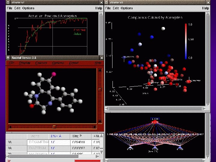
Association Rule Visualization: DBMiner

DBMiner

Association Rule Graph

Clementine (UK, bought by SPSS) The Web Node shows the strength of associations in the data - i. e. how often field values coincide

Multi-Level Association u u Food A descendant of an infrequent itemset cannot be frequent A transaction database can be encoded by dimensions and levels bread milk 2% skim Fraser Sunset wheat white

l Encoding Hierarchical Information in Transaction Database A taxonomy for the relevant data items food milk 2% l . . bread chocolate . into. . generalized_item_id. . . of bar_code Conversion old Mills Wonder Dairyland Foremost . . .

Mining Surprising Temporal Patterns Chakrabarti et al 1990 u Find prevalent rules that hold over large fractions of data u Useful for promotions and store arrangement u Intensively researched Milk and cereal sell together!

Prevalent != Interesting 1995 u Analysts already know about prevalent rules u Interesting rules are those that deviate from prior expectation u Mining’s payoff is in finding surprising phenomena 1998 Zzzz. . . Milk and cereal sell together!

Association Rules - Strengths & Weaknesses u Strengths u Understandable and easy to use u Useful u Weaknesses u Brute u force methods can be expensive (memory and time) Apriori is O(CD), where C = sum of sizes of candidates (2 n possible, n = #items) D = size of database u Association does not necessarily imply correlation u Validation? u Maintenance?

Clustering

Clustering u Group similar items together u Example: sorting laundry u Similar items may have important attributes / functionality in common u Group customers together with similar interests and spending patterns u Form of unsupervised learning u Cluster objects into classes using rule: u Maximize intraclass similarity, minimize interclass similarity

Clustering Techniques u Partition u Enumerate all partitions u Score by some criteria u. K means u Hierarchical u Model based u Hypothesize model for each cluster u Find model that best fits data u Auto. Class, Cobweb

Clustering Goal u u u Suppose you transmit coordinates of points drawn randomly from this dataset Only allowed 2 bits/point What encoder/decoder will lose least information?

Idea One u u Break into grid Decode each bitpair as middle of each grid cell 00 01 10 11

Idea Two u u Break into grid Decode each bitpair as centroid of all data in the grid cell 00 10 01 11

K Means Clustering 1. Ask user how many clusters (e. g. , k=5)

K Means Clustering 1. 2. Ask user how many clusters (e. g. , k=5) Randomly guess k cluster center locations

K Means Clustering 1. 2. 3. Ask user how many clusters (e. g. , k=5) Randomly guess k cluster center locations Each data point finds closest center

K Means Clustering 1. 2. 3. 4. Ask user how many clusters (e. g. , k=5) Randomly guess k cluster center locations Each data point finds closest center Each cluster finds new centroid of its points

K Means Clustering 1. 2. 3. 4. 5. Ask user how many clusters (e. g. , k=5) Randomly guess k cluster center locations Each data point finds closest center Each cluster finds new centroid of its points Repeat until…

K Means Issues u Computationally efficient u Initialization u Termination condition u Distance measure u What should k be?

Hierarchical Clustering 1. Each point is its own cluster

Hierarchical Clustering 1. 2. Each point is its own cluster Find most similar pair of clusters

Hierarchical Clustering 1. 2. 3. Each point is its own cluster Find most similar pair of clusters Merge it into a parent cluster

Hierarchical Clustering 1. 2. 3. 4. Each point is its own cluster Find most similar pair of clusters Merge it into a parent cluster Repeat

Hierarchical Clustering Issues u This was bottom-up clustering (agglomerative clustering) u Can also perform top-down clustering (divisive clustering) u Define similarity between clusters u What is stopping criteria?

Cluster Visualization: IBM u u One row per cluster (# is % size) Charts show fields, ordered by influence Pie: outer ring dist for whole, inner ring for cluster Bar: solid bar for cluster, transparent bar for whole

Structure-based Brushing u User selects region of interest with magenta triangle u User selects level of detail with colored polyline

Spatial Associations FIND SPATIAL ASSOCIATION RULE DESCRIBING "Golf Course" FROM Washington_Golf_courses, Washington WHERE CLOSE_TO(Washington_Golf_courses. Obj, Washington. Obj, "3 km") AND Washington. CFCC <> "D 81" IN RELEVANCE TO Washington_Golf_courses. Obj, Washington. Obj, CFCC SET SUPPORT THRESHOLD 0. 5

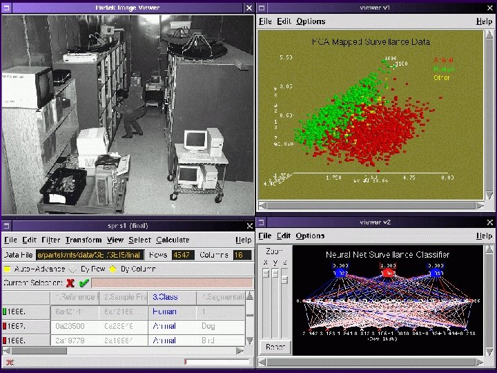
Partek

Conclusions