Modeling with Linear Programming and Graphical Solution Steps

Modeling with Linear Programming and Graphical Solution

Steps in formulating Linear Programming (LP) Models 1. 2. 3. 4. 5. Understand the problem. Identify the decision variables State the objective function as a linear combination of the decision variables. State the constraints as linear combinations of the decision variables. Identify any upper or lower bounds on the decision variables.

LP Model Formulation: A Maximization Example 1 – Product mix problem - Beaver Creek Pottery Company (1 of 4) Beaver Creek Pottery Company employs skilled artisans to produce clay bowls and mugs. The two resources used by the company are special pottery clay and skilled labor. Given these limited resources, the company desires to know how many bowls and mugs to produce each day in order to maximize profit. This is generally referred to as a product mix problem.

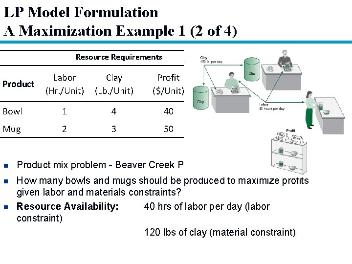
LP Model Formulation A Maximization Example 1 (2 of 4) Resource Requirements Labor (Hr. /Unit) Clay (Lb. /Unit) Profit ($/Unit) Bowl 1 4 40 Mug 2 3 50 Product n Product mix problem - Beaver Creek Pottery Company n How many bowls and mugs should be produced to maximize profits given labor and materials constraints? Resource Availability: 40 hrs of labor per day (labor constraint) 120 lbs of clay (material constraint) n

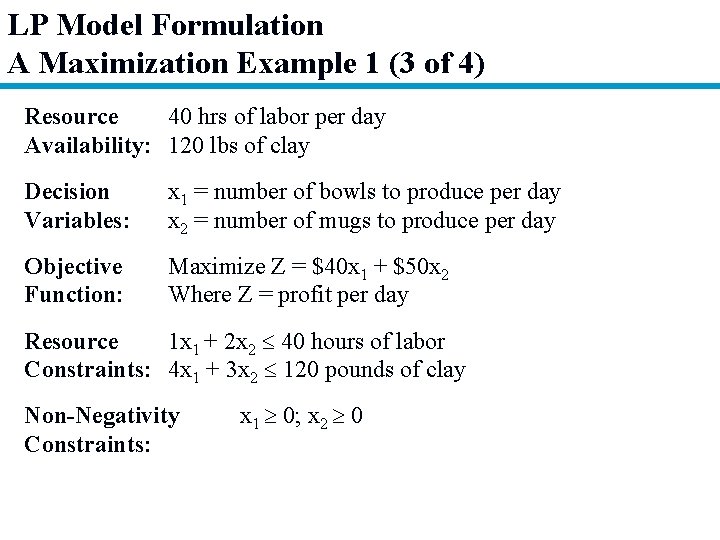
LP Model Formulation A Maximization Example 1 (3 of 4) Resource 40 hrs of labor per day Availability: 120 lbs of clay Decision Variables: x 1 = number of bowls to produce per day x 2 = number of mugs to produce per day Objective Function: Maximize Z = $40 x 1 + $50 x 2 Where Z = profit per day Resource 1 x 1 + 2 x 2 40 hours of labor Constraints: 4 x 1 + 3 x 2 120 pounds of clay Non-Negativity Constraints: x 1 0; x 2 0

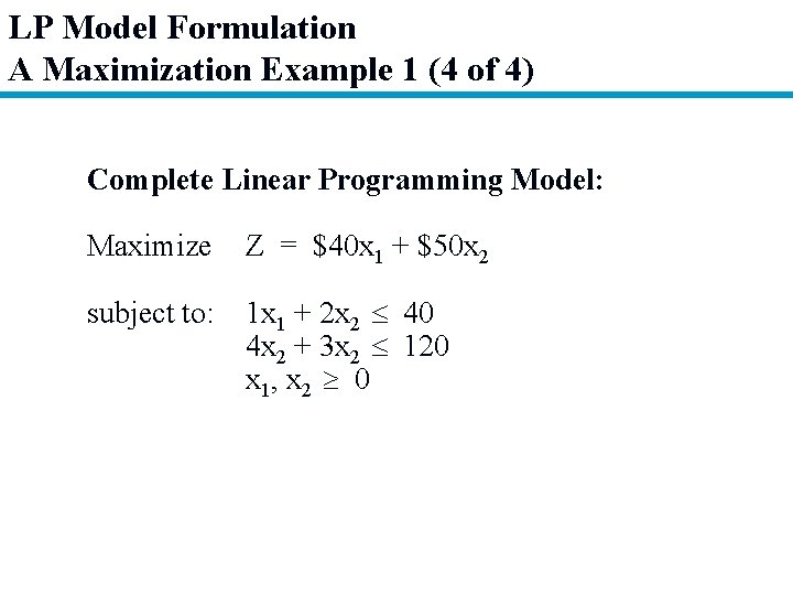
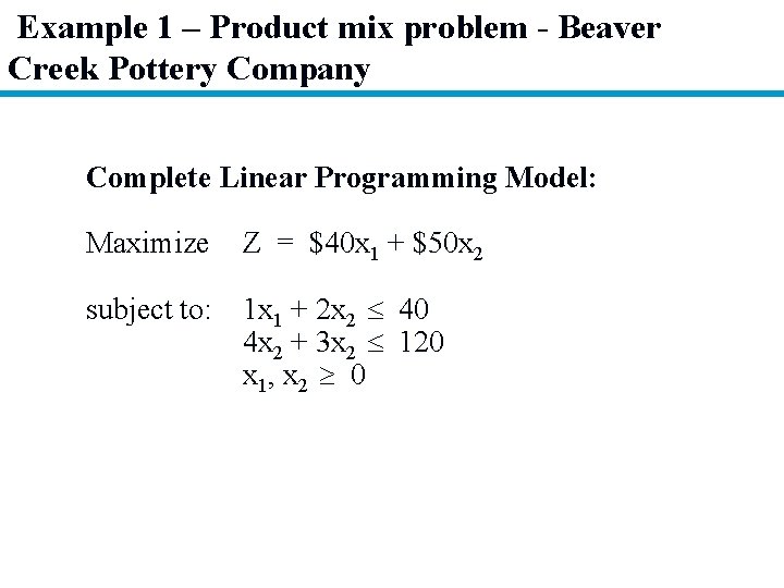
LP Model Formulation A Maximization Example 1 (4 of 4) Complete Linear Programming Model: Maximize Z = $40 x 1 + $50 x 2 subject to: 1 x 1 + 2 x 2 40 4 x 2 + 3 x 2 120 x 1, x 2 0

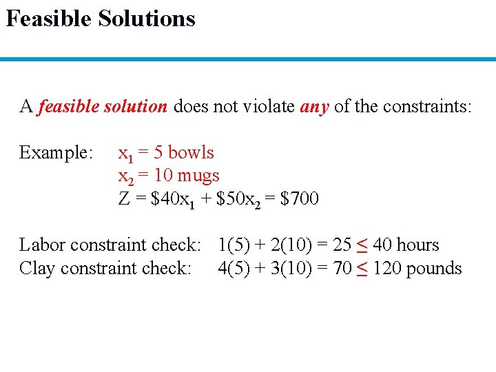
Feasible Solutions A feasible solution does not violate any of the constraints: Example: x 1 = 5 bowls x 2 = 10 mugs Z = $40 x 1 + $50 x 2 = $700 Labor constraint check: 1(5) + 2(10) = 25 ≤ 40 hours Clay constraint check: 4(5) + 3(10) = 70 ≤ 120 pounds

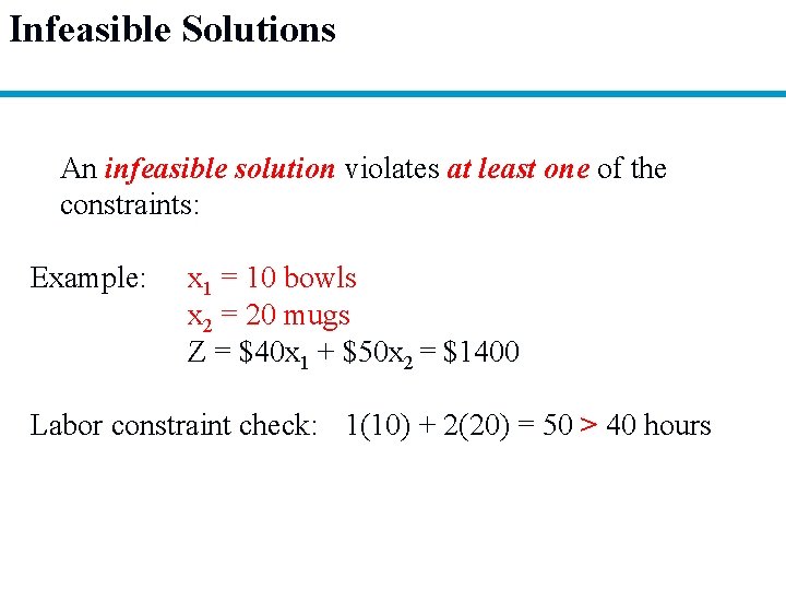
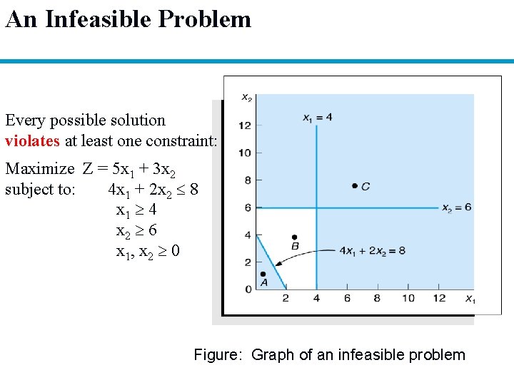
Infeasible Solutions An infeasible solution violates at least one of the constraints: Example: x 1 = 10 bowls x 2 = 20 mugs Z = $40 x 1 + $50 x 2 = $1400 Labor constraint check: 1(10) + 2(20) = 50 > 40 hours

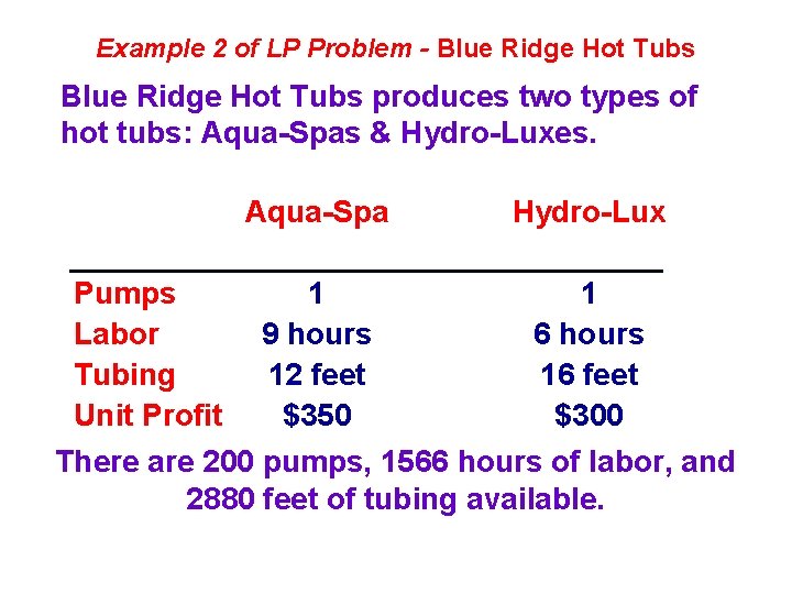
Example 2 of LP Problem - Blue Ridge Hot Tubs produces two types of hot tubs: Aqua-Spas & Hydro-Luxes. Pumps Labor Tubing Unit Profit Aqua-Spa Hydro-Lux 1 9 hours 12 feet $350 1 6 hours 16 feet $300 There are 200 pumps, 1566 hours of labor, and 2880 feet of tubing available.

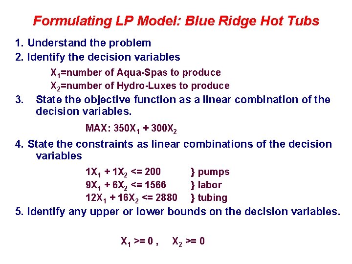
Formulating LP Model: Blue Ridge Hot Tubs 1. Understand the problem 2. Identify the decision variables X 1=number of Aqua-Spas to produce X 2=number of Hydro-Luxes to produce 3. State the objective function as a linear combination of the decision variables. MAX: 350 X 1 + 300 X 2 4. State the constraints as linear combinations of the decision variables 1 X 1 + 1 X 2 <= 200 9 X 1 + 6 X 2 <= 1566 12 X 1 + 16 X 2 <= 2880 } pumps } labor } tubing 5. Identify any upper or lower bounds on the decision variables. X 1 >= 0 , X 2 >= 0

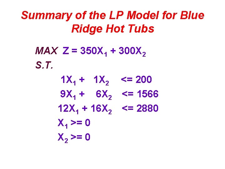
Summary of the LP Model for Blue Ridge Hot Tubs MAX Z = 350 X 1 + 300 X 2 S. T. 1 X 1 + 1 X 2 <= 200 9 X 1 + 6 X 2 <= 1566 12 X 1 + 16 X 2 <= 2880 X 1 >= 0 X 2 >= 0

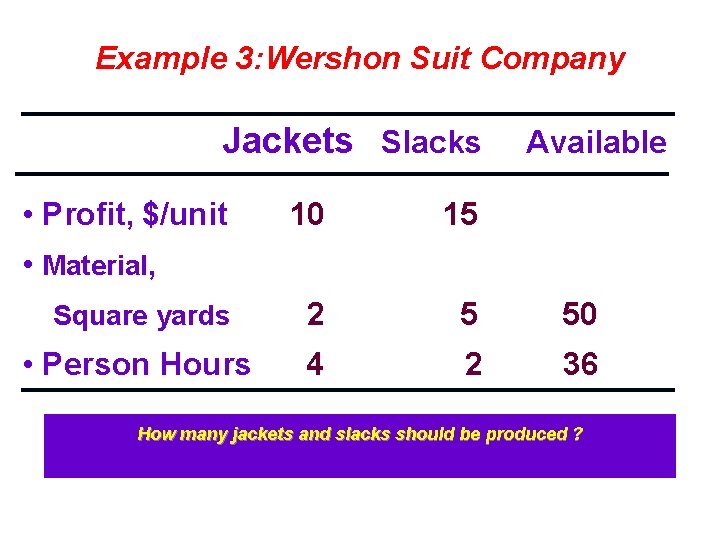
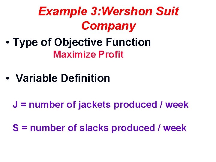
Example 3: Wershon Suit Company Jackets Slacks Available • Profit, $/unit • Material, 10 15 Square yards 2 5 50 • Person Hours 4 2 36 How many jackets and slacks should be produced ?

Example 3: Wershon Suit Company • Type of Objective Function Maximize Profit • Variable Definition J = number of jackets produced / week S = number of slacks produced / week

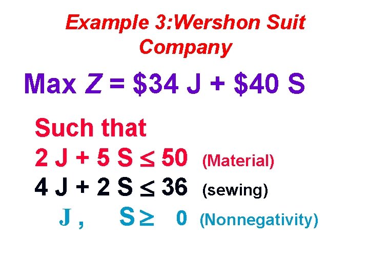
Example 3: Wershon Suit Company Max Z = $34 J + $40 S Such that 2 J + 5 S 50 4 J + 2 S 36 J , S 0 (Material) (sewing) (Nonnegativity)

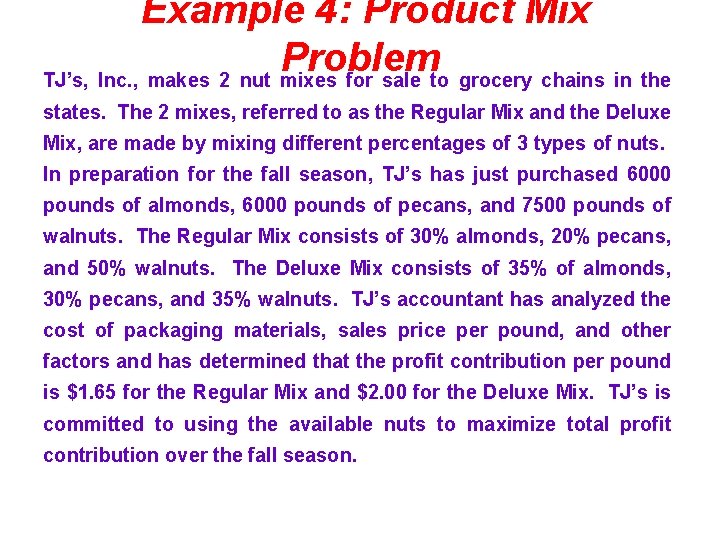
Example 4: Product Mix Problem TJ’s, Inc. , makes 2 nut mixes for sale to grocery chains in the states. The 2 mixes, referred to as the Regular Mix and the Deluxe Mix, are made by mixing different percentages of 3 types of nuts. In preparation for the fall season, TJ’s has just purchased 6000 pounds of almonds, 6000 pounds of pecans, and 7500 pounds of walnuts. The Regular Mix consists of 30% almonds, 20% pecans, and 50% walnuts. The Deluxe Mix consists of 35% of almonds, 30% pecans, and 35% walnuts. TJ’s accountant has analyzed the cost of packaging materials, sales price per pound, and other factors and has determined that the profit contribution per pound is $1. 65 for the Regular Mix and $2. 00 for the Deluxe Mix. TJ’s is committed to using the available nuts to maximize total profit contribution over the fall season.

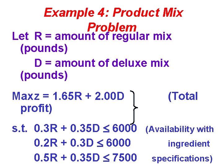
Example 4: Product Mix Problem Let R = amount of regular mix (pounds) D = amount of deluxe mix (pounds) Maxz = 1. 65 R + 2. 00 D profit) s. t. 0. 3 R + 0. 35 D 6000 0. 2 R + 0. 3 D 6000 0. 5 R + 0. 35 D 7500 (Total (Availability with ingredient specifications)

Example 5: Transportation Problem n A product is to be shipped in the amounts al, a 2, . . . , am from m shipping origins and received in amounts bl, b 2, . . . , bn at each of n shipping destinations. n The cost of shipping a unit from the ith origin to the jth destination is known for all combinations of origins and destinations. n The problem is to determine the amount to be shipped from each origin to each destination such that the total cost of transportation is a minimum.

Transportation Problem – Example 5 The Zephyr Television Company ships televisions from three warehouses to three retail stores on a monthly basis. Each warehouse has a fixed supply per month, and each store has a fixed demand per month. The manufacturer wants to know the number of television sets to ship from each warehouse to each store in order to minimize the total cost of transportation.

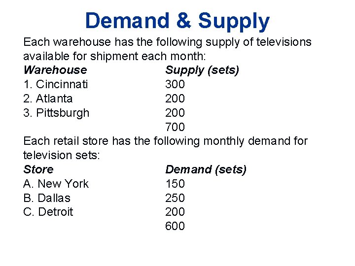
Demand & Supply Each warehouse has the following supply of televisions available for shipment each month: Warehouse Supply (sets) 1. Cincinnati 300 2. Atlanta 200 3. Pittsburgh 200 700 Each retail store has the following monthly demand for television sets: Store Demand (sets) A. New York 150 B. Dallas 250 C. Detroit 200 600

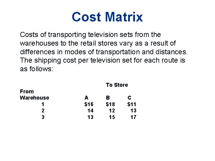
Cost Matrix Costs of transporting television sets from the warehouses to the retail stores vary as a result of differences in modes of transportation and distances. The shipping cost per television set for each route is as follows: To Store From Warehouse 1 2 3 A $16 14 13 B $18 12 15 C $11 13 17

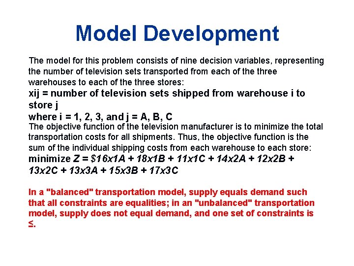
Model Development The model for this problem consists of nine decision variables, representing the number of television sets transported from each of the three warehouses to each of the three stores: xij = number of television sets shipped from warehouse i to store j where i = 1, 2, 3, and j = A, B, C The objective function of the television manufacturer is to minimize the total transportation costs for all shipments. Thus, the objective function is the sum of the individual shipping costs from each warehouse to each store: minimize Z = $16 x 1 A + 18 x 1 B + 11 x 1 C + 14 x 2 A + 12 x 2 B + 13 x 2 C + 13 x 3 A + 15 x 3 B + 17 x 3 C In a "balanced" transportation model, supply equals demand such that all constraints are equalities; in an "unbalanced" transportation model, supply does not equal demand, and one set of constraints is ≤.

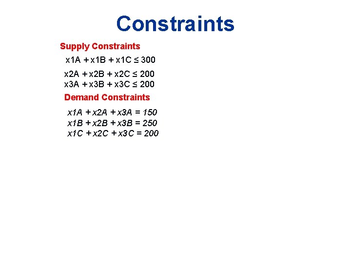
Constraints Supply Constraints x 1 A + x 1 B + x 1 C ≤ 300 x 2 A + x 2 B + x 2 C ≤ 200 x 3 A + x 3 B + x 3 C ≤ 200 Demand Constraints x 1 A + x 2 A + x 3 A = 150 x 1 B + x 2 B + x 3 B = 250 x 1 C + x 2 C + x 3 C = 200

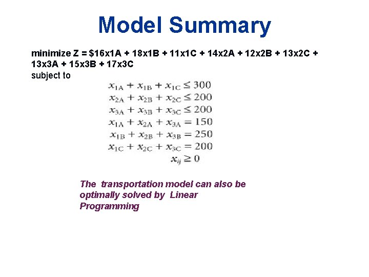
Model Summary minimize Z = $16 x 1 A + 18 x 1 B + 11 x 1 C + 14 x 2 A + 12 x 2 B + 13 x 2 C + 13 x 3 A + 15 x 3 B + 17 x 3 C subject to The transportation model can also be optimally solved by Linear Programming

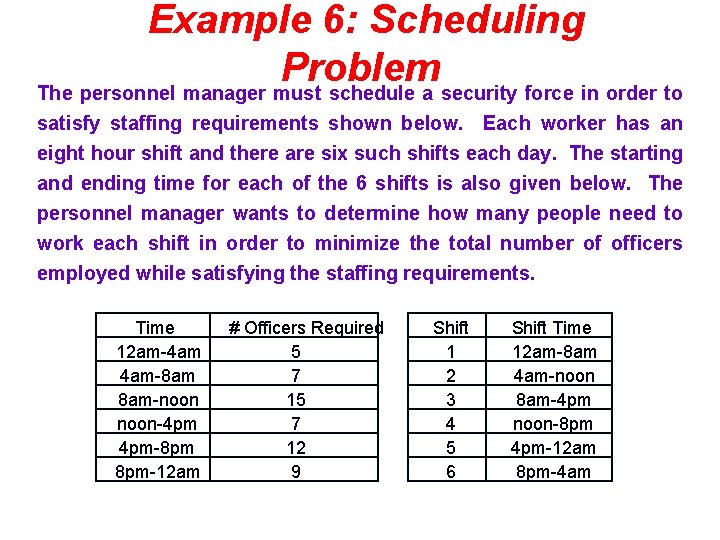
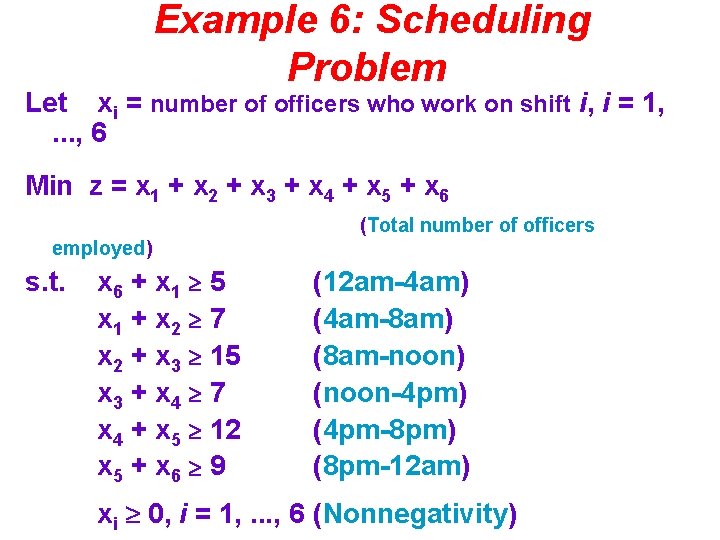
Example 6: Scheduling Problem The personnel manager must schedule a security force in order to satisfy staffing requirements shown below. Each worker has an eight hour shift and there are six such shifts each day. The starting and ending time for each of the 6 shifts is also given below. The personnel manager wants to determine how many people need to work each shift in order to minimize the total number of officers employed while satisfying the staffing requirements. Time 12 am-4 am 4 am-8 am 8 am-noon-4 pm 4 pm-8 pm 8 pm-12 am # Officers Required 5 7 12 9 Shift 1 2 3 4 5 6 Shift Time 12 am-8 am 4 am-noon 8 am-4 pm noon-8 pm 4 pm-12 am 8 pm-4 am

Example 6: Scheduling Problem Let xi = number of officers who work on shift i, i = 1, . . . , 6 Min z = x 1 + x 2 + x 3 + x 4 + x 5 + x 6 (Total number of officers employed) s. t. x 6 + x 1 5 x 1 + x 2 7 x 2 + x 3 15 x 3 + x 4 7 x 4 + x 5 12 x 5 + x 6 9 (12 am-4 am) (4 am-8 am) (8 am-noon) (noon-4 pm) (4 pm-8 pm) (8 pm-12 am) xi 0, i = 1, . . . , 6 (Nonnegativity)

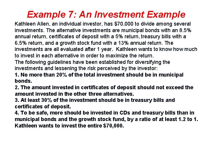
Example 7: An Investment Example Kathleen Allen, an individual investor, has $70, 000 to divide among several investments. The alternative investments are municipal bonds with an 8. 5% annual return, certificates of deposit with a 5% return, treasury bills with a 6. 5% return, and a growth stock fund with a 13% annual return. The investments are all evaluated after 1 year. Kathleen wants to know how much to invest in each alternative in order to maximize the return. The following guidelines have been established for diversifying the investments and lessening the risk perceived by the investor: 1. No more than 20% of the total investment should be in municipal bonds. 2. The amount invested in certificates of deposit should not exceed the amount invested in the other three alternatives. 3. At least 30% of the investment should be in treasury bills and certificates of deposit. 4. To be safe, more should be invested in CDs and treasury bills than in municipal bonds and the growth stock fund, by a ratio of at least 1. 2 to 1. Kathleen wants to invest the entire $70, 000.

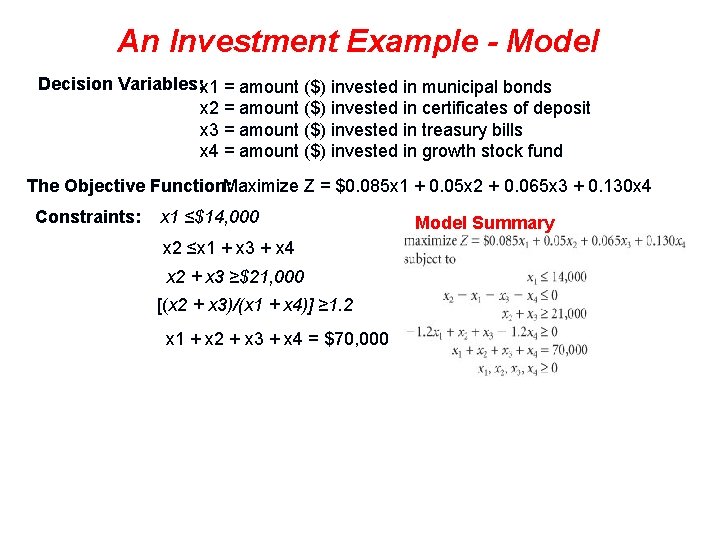
An Investment Example - Model Decision Variables: x 1 = amount ($) invested in municipal bonds x 2 = amount ($) invested in certificates of deposit x 3 = amount ($) invested in treasury bills x 4 = amount ($) invested in growth stock fund The Objective Function: Maximize Z = $0. 085 x 1 + 0. 05 x 2 + 0. 065 x 3 + 0. 130 x 4 Constraints: x 1 ≤$14, 000 x 2 ≤x 1 + x 3 + x 4 x 2 + x 3 ≥$21, 000 [(x 2 + x 3)/(x 1 + x 4)] ≥ 1. 2 x 1 + x 2 + x 3 + x 4 = $70, 000 Model Summary

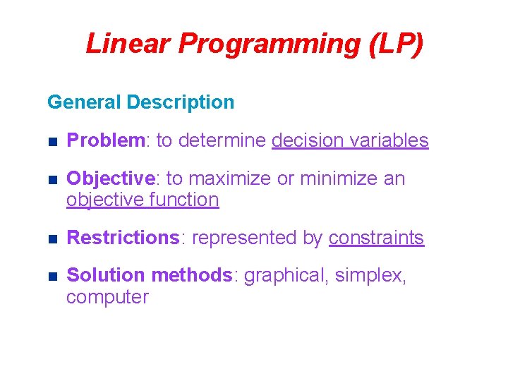
Linear Programming (LP) General Description n Problem: to determine decision variables n Objective: to maximize or minimize an objective function n Restrictions: represented by constraints n Solution methods: graphical, simplex, computer

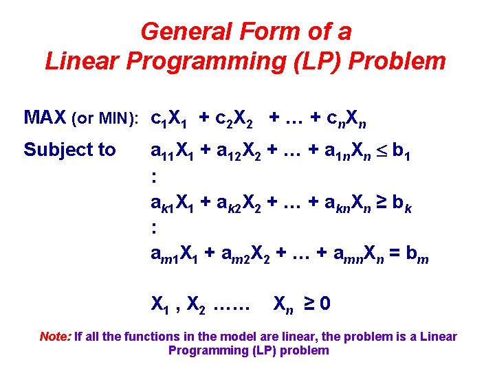
General Form of a Linear Programming (LP) Problem MAX (or MIN): c 1 X 1 + c 2 X 2 + … + cn. Xn Subject to a 11 X 1 + a 12 X 2 + … + a 1 n. Xn b 1 : ak 1 X 1 + ak 2 X 2 + … + akn. Xn ≥ bk : am 1 X 1 + am 2 X 2 + … + amn. Xn = bm X 1 , X 2 …… Xn ≥ 0 Note: If all the functions in the model are linear, the problem is a Linear Programming (LP) problem

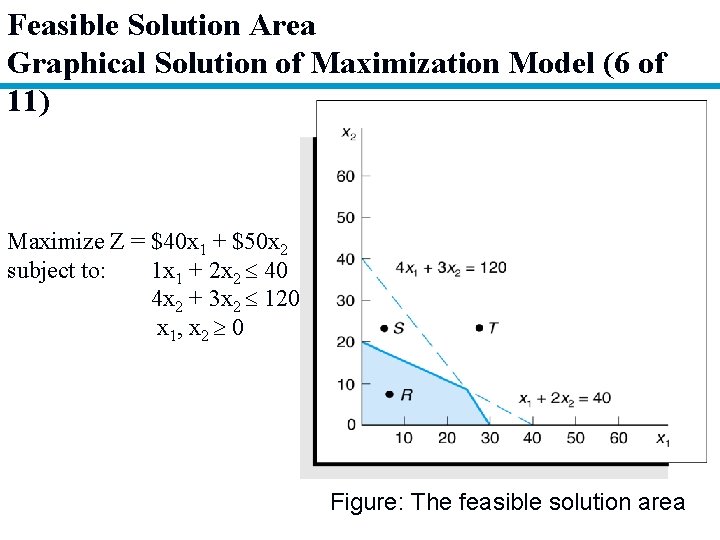
Graphical Solution of LP Models n Graphical solution is limited to linear programming models containing only two decision variables. n Graphical methods provide visualization of how a solution for a linear programming problem is obtained.

Example 1 – Product mix problem - Beaver Creek Pottery Company Complete Linear Programming Model: Maximize Z = $40 x 1 + $50 x 2 subject to: 1 x 1 + 2 x 2 40 4 x 2 + 3 x 2 120 x 1, x 2 0

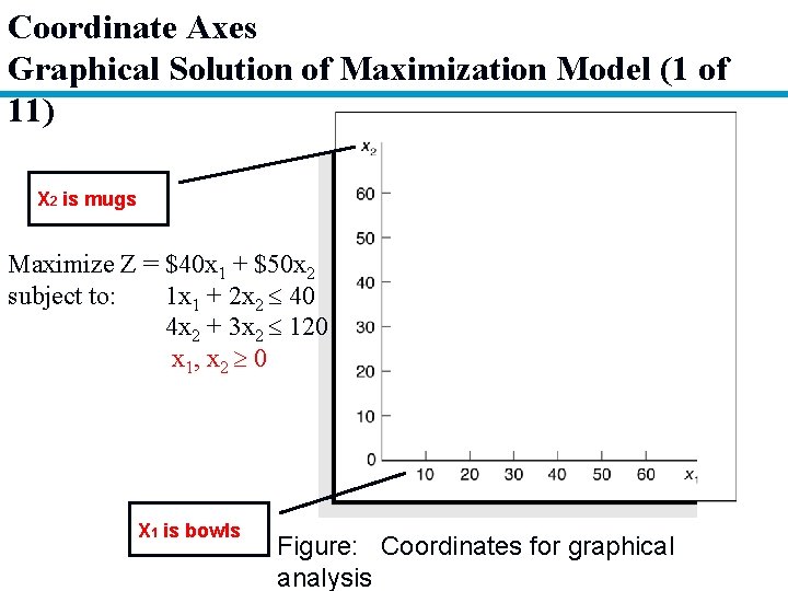
Coordinate Axes Graphical Solution of Maximization Model (1 of 11) X 2 is mugs Maximize Z = $40 x 1 + $50 x 2 subject to: 1 x 1 + 2 x 2 40 4 x 2 + 3 x 2 120 x 1, x 2 0 X 1 is bowls Figure: Coordinates for graphical analysis

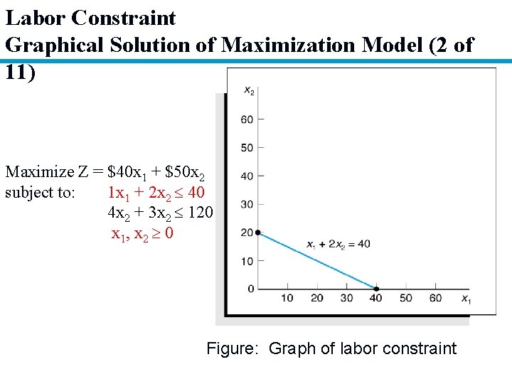
Labor Constraint Graphical Solution of Maximization Model (2 of 11) Maximize Z = $40 x 1 + $50 x 2 subject to: 1 x 1 + 2 x 2 40 4 x 2 + 3 x 2 120 x 1, x 2 0 Figure: Graph of labor constraint

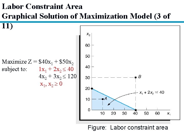
Labor Constraint Area Graphical Solution of Maximization Model (3 of 11) Maximize Z = $40 x 1 + $50 x 2 subject to: 1 x 1 + 2 x 2 40 4 x 2 + 3 x 2 120 x 1, x 2 0 Figure: Labor constraint area

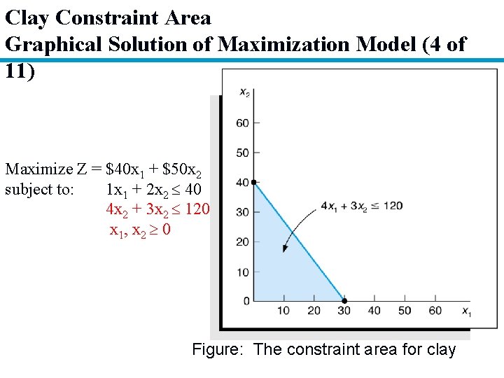
Clay Constraint Area Graphical Solution of Maximization Model (4 of 11) Maximize Z = $40 x 1 + $50 x 2 subject to: 1 x 1 + 2 x 2 40 4 x 2 + 3 x 2 120 x 1, x 2 0 Figure: The constraint area for clay

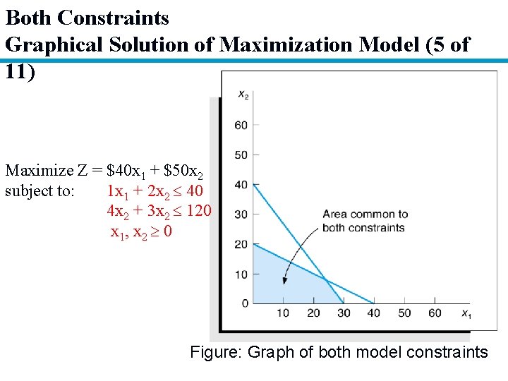
Both Constraints Graphical Solution of Maximization Model (5 of 11) Maximize Z = $40 x 1 + $50 x 2 subject to: 1 x 1 + 2 x 2 40 4 x 2 + 3 x 2 120 x 1, x 2 0 Figure: Graph of both model constraints

Feasible Solution Area Graphical Solution of Maximization Model (6 of 11) Maximize Z = $40 x 1 + $50 x 2 subject to: 1 x 1 + 2 x 2 40 4 x 2 + 3 x 2 120 x 1, x 2 0 Figure: The feasible solution area

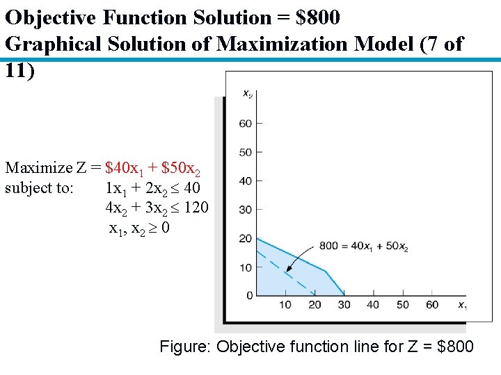
Objective Function Solution = $800 Graphical Solution of Maximization Model (7 of 11) Maximize Z = $40 x 1 + $50 x 2 subject to: 1 x 1 + 2 x 2 40 4 x 2 + 3 x 2 120 x 1, x 2 0 Figure: Objective function line for Z = $800

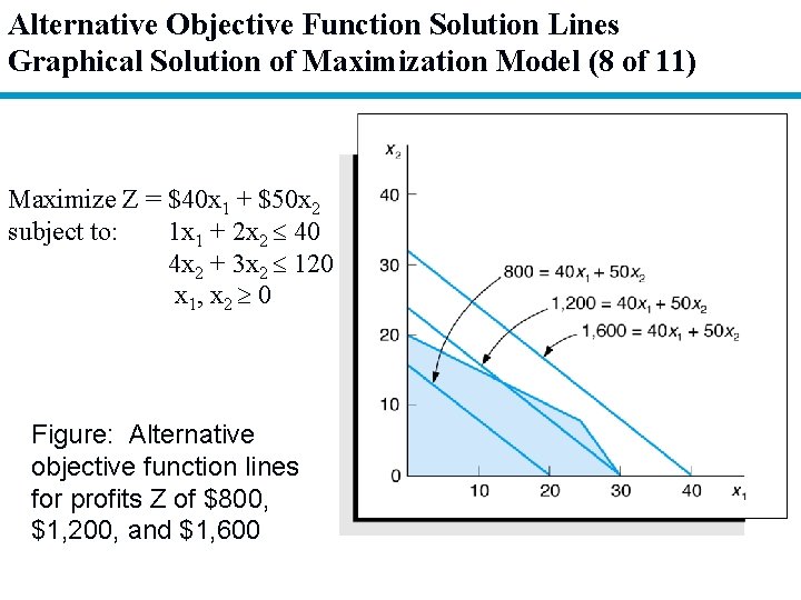
Alternative Objective Function Solution Lines Graphical Solution of Maximization Model (8 of 11) Maximize Z = $40 x 1 + $50 x 2 subject to: 1 x 1 + 2 x 2 40 4 x 2 + 3 x 2 120 x 1, x 2 0 Figure: Alternative objective function lines for profits Z of $800, $1, 200, and $1, 600

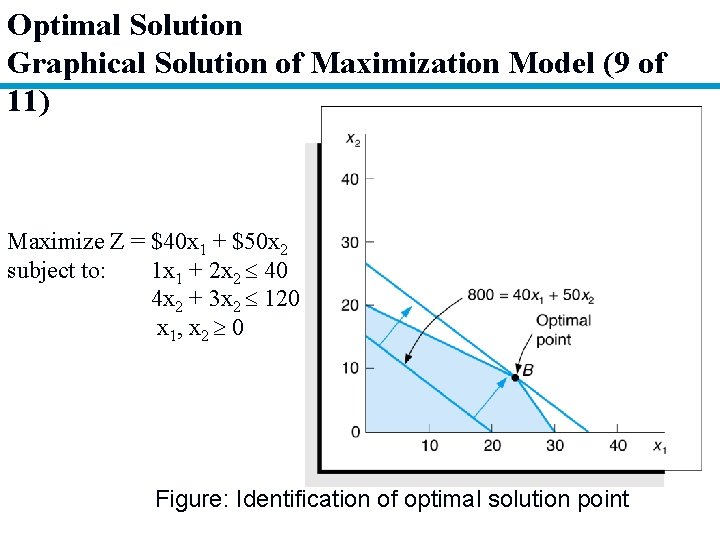
Optimal Solution Graphical Solution of Maximization Model (9 of 11) Maximize Z = $40 x 1 + $50 x 2 subject to: 1 x 1 + 2 x 2 40 4 x 2 + 3 x 2 120 x 1, x 2 0 Figure: Identification of optimal solution point

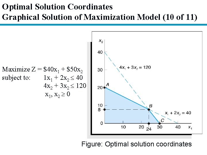
Optimal Solution Coordinates Graphical Solution of Maximization Model (10 of 11) Maximize Z = $40 x 1 + $50 x 2 subject to: 1 x 1 + 2 x 2 40 4 x 2 + 3 x 2 120 x 1, x 2 0 Figure: Optimal solution coordinates

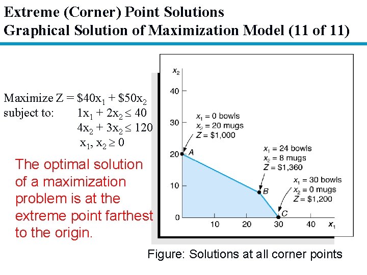
Extreme (Corner) Point Solutions Graphical Solution of Maximization Model (11 of 11) Maximize Z = $40 x 1 + $50 x 2 subject to: 1 x 1 + 2 x 2 40 4 x 2 + 3 x 2 120 x 1, x 2 0 The optimal solution of a maximization problem is at the extreme point farthest to the origin. Figure: Solutions at all corner points

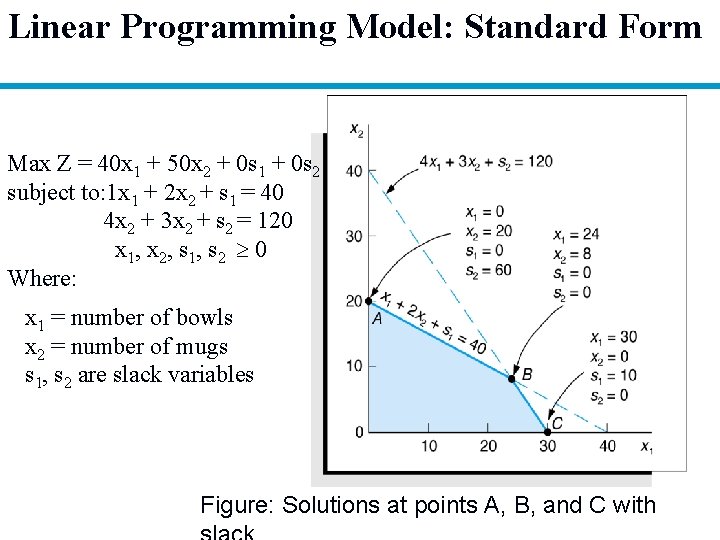
Slack Variables n n Standard form requires that all constraints be in the form of equations (equalities). A slack variable is added to a constraint to convert it to an equation (=). n A slack variable typically represents an unused resource. n A slack variable contributes nothing to the objective function value.

Linear Programming Model: Standard Form Max Z = 40 x 1 + 50 x 2 + 0 s 1 + 0 s 2 subject to: 1 x 1 + 2 x 2 + s 1 = 40 4 x 2 + 3 x 2 + s 2 = 120 x 1, x 2, s 1, s 2 0 Where: x 1 = number of bowls x 2 = number of mugs s 1, s 2 are slack variables Figure: Solutions at points A, B, and C with

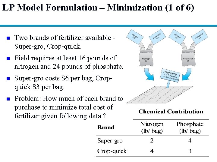
LP Model Formulation – Minimization (1 of 6) n Two brands of fertilizer available Super-gro, Crop-quick. n Field requires at least 16 pounds of nitrogen and 24 pounds of phosphate. n Super-gro costs $6 per bag, Cropquick $3 per bag. n Problem: How much of each brand to purchase to minimize total cost of fertilizer given following data ?

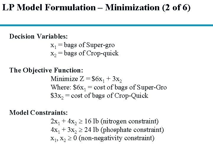
LP Model Formulation – Minimization (2 of 6) Decision Variables: x 1 = bags of Super-gro x 2 = bags of Crop-quick The Objective Function: Minimize Z = $6 x 1 + 3 x 2 Where: $6 x 1 = cost of bags of Super-Gro $3 x 2 = cost of bags of Crop-Quick Model Constraints: 2 x 1 + 4 x 2 16 lb (nitrogen constraint) 4 x 1 + 3 x 2 24 lb (phosphate constraint) x 1, x 2 0 (non-negativity constraint)

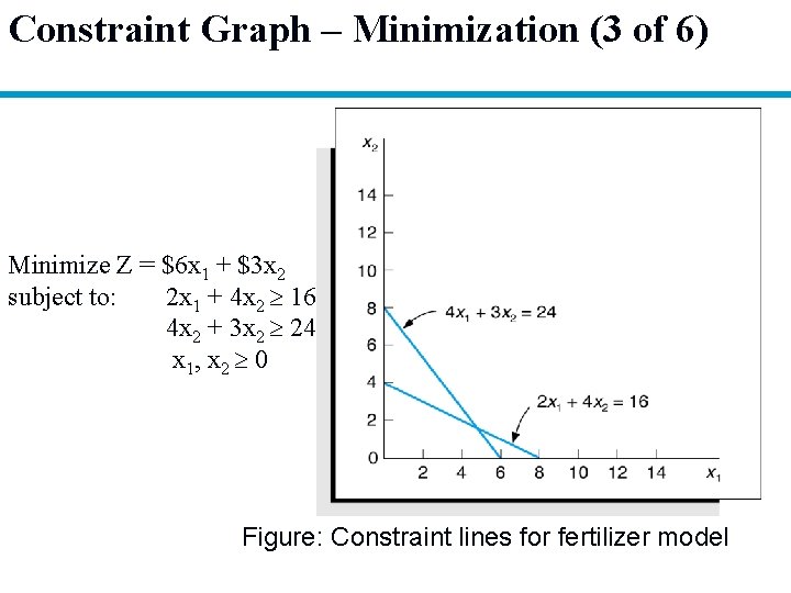
Constraint Graph – Minimization (3 of 6) Minimize Z = $6 x 1 + $3 x 2 subject to: 2 x 1 + 4 x 2 16 4 x 2 + 3 x 2 24 x 1, x 2 0 Figure: Constraint lines for fertilizer model

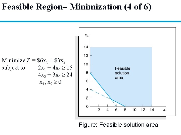
Feasible Region– Minimization (4 of 6) Minimize Z = $6 x 1 + $3 x 2 subject to: 2 x 1 + 4 x 2 16 4 x 2 + 3 x 2 24 x 1, x 2 0 Figure: Feasible solution area

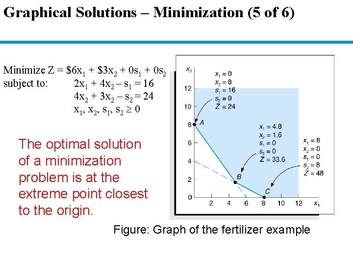
Graphical Solutions – Minimization (5 of 6) Minimize Z = $6 x 1 + $3 x 2 + 0 s 1 + 0 s 2 subject to: 2 x 1 + 4 x 2 – s 1 = 16 4 x 2 + 3 x 2 – s 2 = 24 x 1, x 2, s 1, s 2 0 The optimal solution of a minimization problem is at the extreme point closest to the origin. Figure: Graph of the fertilizer example

Surplus Variables – Minimization (6 of 6) n A surplus variable is subtracted from a constraint to convert it to an equation (=). n A surplus variable represents an excess above a constraint requirement level. n A surplus variable contributes nothing to the calculated value of the objective function. n Subtracting surplus variables in the farmer problem constraints: 2 x 1 + 4 x 2 - s 1 = 16 (nitrogen) 4 x 1 + 3 x 2 - s 2 = 24 (phosphate)

Irregular Types of Linear Programming Problems For some linear programming models, the general rules do not apply. Special types of problems include those with: § Multiple optimal solutions § Infeasible solutions § Unbounded solutions

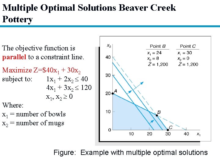
Multiple Optimal Solutions Beaver Creek Pottery The objective function is parallel to a constraint line. Maximize Z=$40 x 1 + 30 x 2 subject to: 1 x 1 + 2 x 2 40 4 x 1 + 3 x 2 120 x 1, x 2 0 Where: x 1 = number of bowls x 2 = number of mugs Figure: Example with multiple optimal solutions

An Infeasible Problem Every possible solution violates at least one constraint: Maximize Z = 5 x 1 + 3 x 2 subject to: 4 x 1 + 2 x 2 8 x 1 4 x 2 6 x 1, x 2 0 Figure: Graph of an infeasible problem

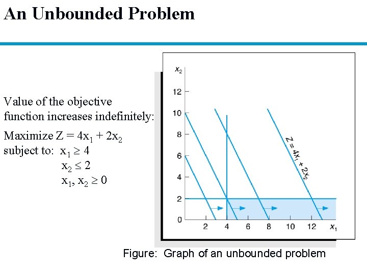
An Unbounded Problem Value of the objective function increases indefinitely: Maximize Z = 4 x 1 + 2 x 2 subject to: x 1 4 x 2 2 x 1, x 2 0 Figure: Graph of an unbounded problem

Characteristics of Linear Programming Problems n n n A decision amongst alternative courses of action is required. The decision is represented in the model by decision variables. The problem encompasses a goal, expressed as an objective function, that the decision maker wants to achieve. Restrictions (represented by constraints) exist that limit the extent of achievement of the objective. The objective and constraints must be definable by linear mathematical functional relationships.

Properties of Linear Programming Models n Proportionality - The rate of change (slope) of the objective function and constraint equations is constant. n Additivity - Terms in the objective function and constraint equations must be additive. n Divisibility - Decision variables can take on any fractional value and are therefore continuous as opposed to integer in nature. n Certainty - Values of all the model parameters are assumed to be known with certainty (non-probabilistic).