MCMC and SMC for Nonlinear Time Series Models

MCMC and SMC for Nonlinear Time Series Models Chiranjit Mukherjee STA 395 Talk Department of Statistical Science, Duke University February 16, 2009 1

Outline 1. Problem Statement 2. Markov Chain Monte Carlo Dynamic Linear Models, Forward Filtering Backward Sampling, Nonlinear Models, Mixture of Gaussians, Approximate FFBS as a proposal to Metropolis-Hastings 3. Sequential Monte Carlo Importance Sampling, Sequential Importance Sampling, Optimal Proposal, Resampling, Auxiliary Particle Filters, Parameter Degeneracy, Marginal Likelihood Calculation, Issues with Resampling, Scalability of SMC techniques 4. Minimal Quorum Sensing Model Background, Differential Equations Model, Discretized Version, Features 5. Results 6. Summery 7. References 2

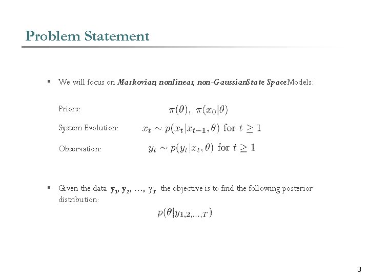
Problem Statement § We will focus on Markovian, nonlinear, non-Gaussian. State Space Models: Priors: System Evolution: Observation: § Given the data y 1, y 2, …, y. T the objective is to find the following posterior distribution: 3

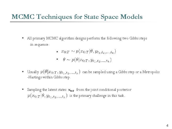
MCMC Techniques for State Space Models § All primary MCMC algorithm designs perform the following two Gibbs steps in sequence: § § § Usually -Hastings within Gibbs step. can be sampled using a Gibbs step or a Metropolis § Sampling the latent states x 0: T from the joint conditional posterior is the primary challenge in this task. 4

Dynamic Linear Models [West and Harrison, 1997] where all known. One can sample from the joint distribution of x 0: T given and using a Forward Filtering Backward Sampling. Algorithm. [Carter & Kohn, 1994] 5

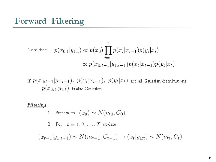
Forward Filtering Note that: If are all Gaussian distributions, is also Gaussian. Filtering: 1. Start with 2. For update 6

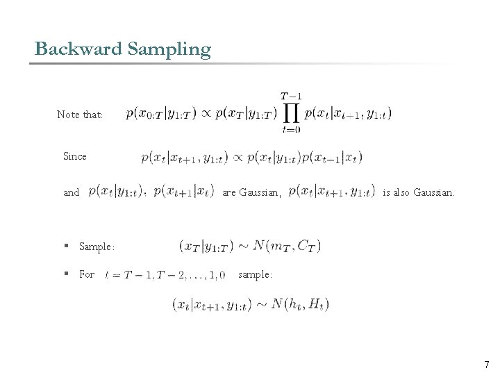
Backward Sampling Note that: Since and are Gaussian, is also Gaussian. § Sample: § For sample: 7

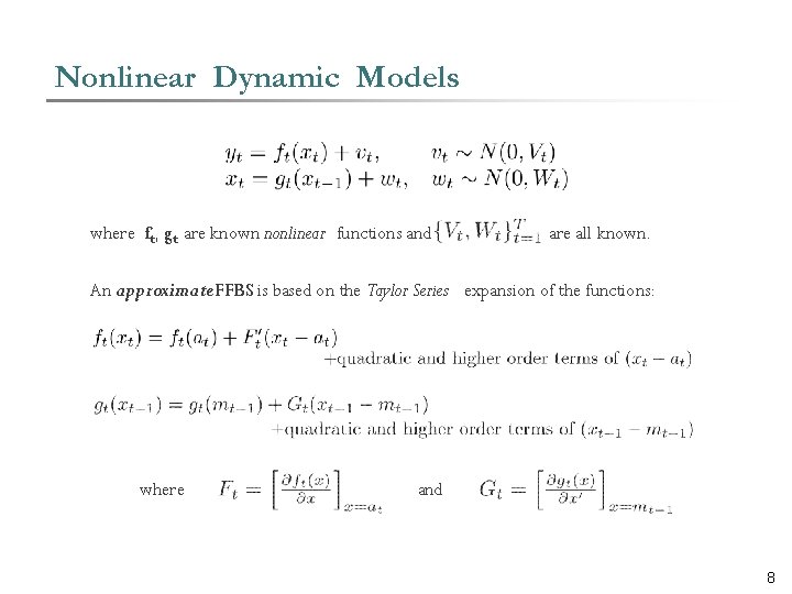
Nonlinear Dynamic Models where ft, gt are known nonlinear functions and are all known. An approximate FFBS is based on the Taylor Series expansion of the functions: where and 8

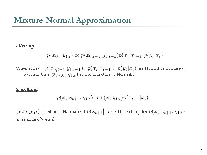
Mixture Normal Approximation Filtering: When each of Normals then are Normal or mixture of is also a mixture of Normals. Smoothing: is mixture Normal and is a mixture Normal. is Normal implies 9

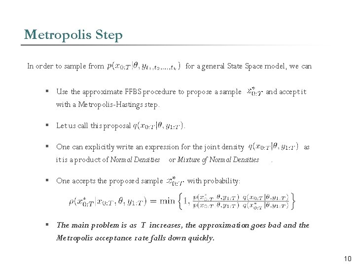
Metropolis Step In order to sample from for a general State Space model, we can § Use the approximate FFBS procedure to propose a sample with a Metropolis-Hastings step. § Let us call this proposal . § One can explicitly write an expression for the joint density it is a product of Normal Densities or Mixture of Normal Densities § One accepts the proposed sample and accept it as. with probability: § The main problem is as T increases, the approximation goes bad and the Metropolis acceptance rate falls down quickly. 10

Sequential Monte Carlo 11

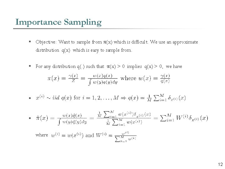
Importance Sampling § Objective: Want to sample from ¼(x) which is difficult. We use an approximate distribution q(x) which is easy to sample from. § For any distribution q(. ) such that ¼(x) > 0 implies q(x) > 0, we have § § where 12

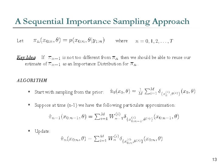
A Sequential Importance Sampling Approach Let where Key Idea: If estimate of is not too different from then we should be able to reuse our as an Importance Distribution for. ALGORITHM § Start with sampling from the prior: § Suppose at time (n-1) we have the following particulate approximation: § Update: 13

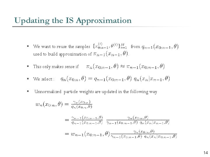
Updating the IS Approximation § We want to reuse the samples used to build approximation of from. § This only makes sense if § We select : § Unnormalized particle weights are updated in the following way 14

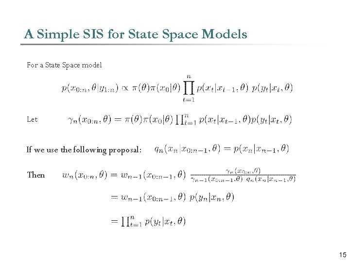
A Simple SIS for State Space Models For a State Space model Let If we use the following proposal: Then 15

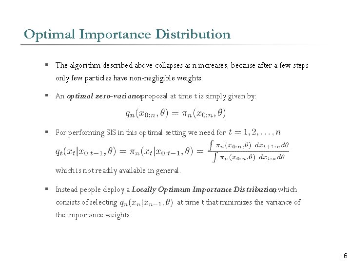
Optimal Importance Distribution § The algorithm described above collapses as n increases, because after a few steps only few particles have non-negligible weights. § An optimal zero-varianceproposal at time t is simply given by: § For performing SIS in this optimal setting we need for which is not readily available in general. § Instead people deploy a Locally Optimum Importance Distribution, which consists of selecting at time t that minimizes the variance of the importance weights. 16

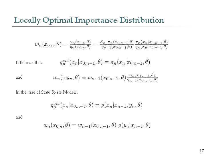
Locally Optimal Importance Distribution It follows that: and In the case of State Space Models: and 17

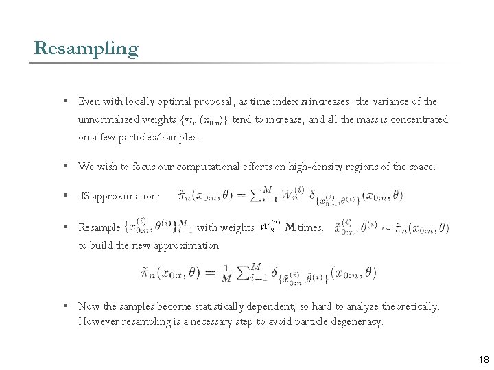
Resampling § Even with locally optimal proposal, as time index n increases, the variance of the unnormalized weights {wn (x 0: n)} tend to increase, and all the mass is concentrated on a few particles/samples. § We wish to focus our computational efforts on high-density regions of the space. § IS approximation: § Resample with weights to build the new approximation M times: § Now the samples become statistically dependent, so hard to analyze theoretically. However resampling is a necessary step to avoid particle degeneracy. 18

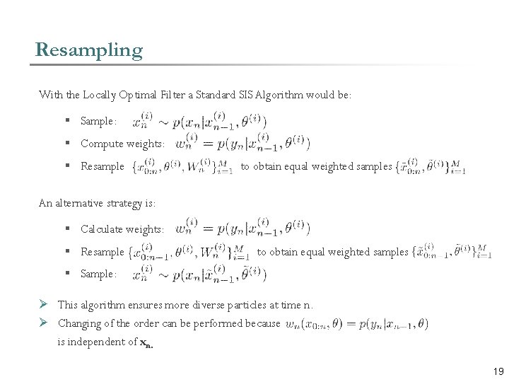
Resampling With the Locally Optimal Filter a Standard SIS Algorithm would be: § Sample: § Compute weights: § Resample to obtain equal weighted samples An alternative strategy is: § Calculate weights: § Resample to obtain equal weighted samples § Sample: Ø This algorithm ensures more diverse particles at time n. Ø Changing of the order can be performed because is independent of xn. 19

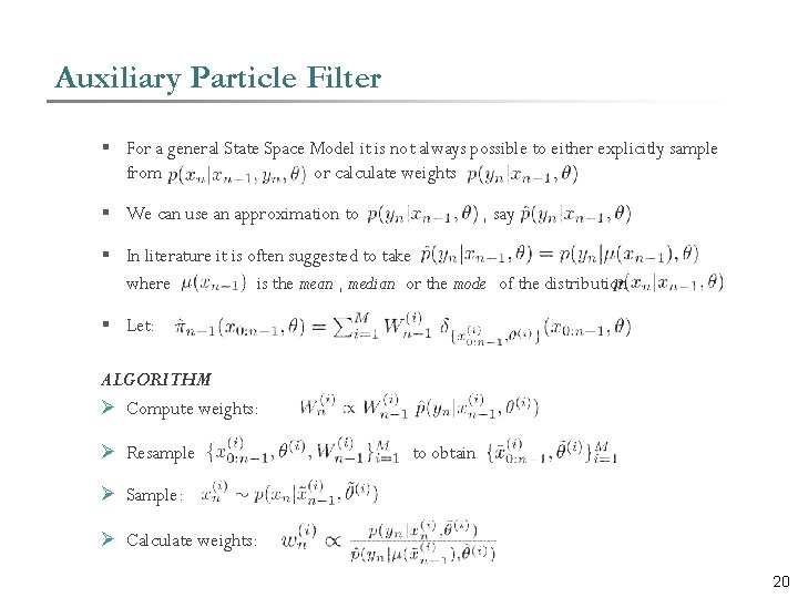
Auxiliary Particle Filter § For a general State Space Model it is not always possible to either explicitly sample from or calculate weights § We can use an approximation to , say § In literature it is often suggested to take where is the mean , median or the mode of the distribution § Let: ALGORITHM Ø Compute weights: Ø Resample to obtain Ø Sample: Ø Calculate weights: 20

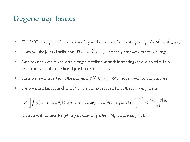
Degeneracy Issues § The SMC strategy performs remarkably well in terms of estimating marginals § However the joint distribution § One can not hope to estimate a target distribution with increasing dimension with fixed precision when the number of particles remains fixed. § Since we are interested in the marginal § For bounded functions Á and p>1, we can expect results of the following form is poorly estimated when n is large. , SMC serves well for our purpose. if the model has nice forgetting/mixing properties. ML is increasing in L. 21

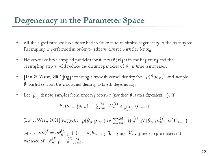
Degeneracy in the Parameter Space § All the algorithms we have described so far tries to minimize degeneracy in the state space. Resampling is performed in order to achieve diverse particles for xn. § However we have sampled particles for µ ~ ¼ (µ) right in the beginning and the resampling step would reduce the distinct particles of µ as time n increases. § [Liu & West, 2001]suggests using a smooth kernel density for µ particles from the smoothed density to break degeneracy. § Let and sample denote samples from time n posterior (not that µ is time dependent ). If [Liu & West, 2001] suggests: where variance of ; and are sample mean and . 22

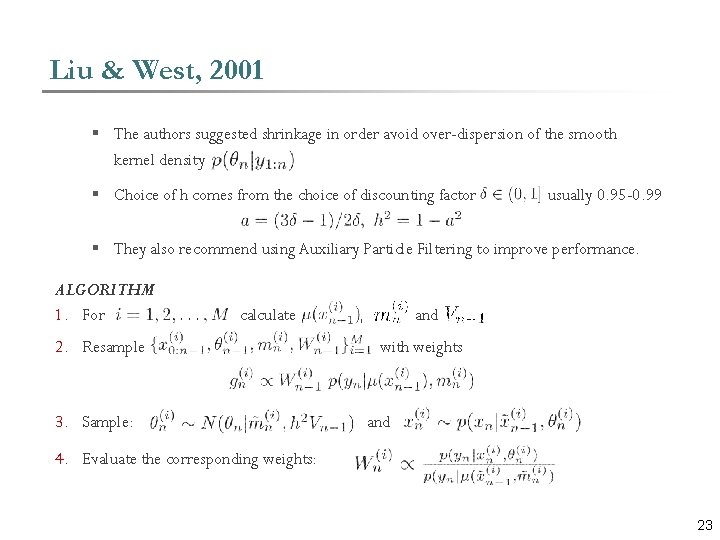
Liu & West, 2001 § The authors suggested shrinkage in order avoid over-dispersion of the smooth kernel density § Choice of h comes from the choice of discounting factor usually 0. 95 -0. 99 § They also recommend using Auxiliary Particle Filtering to improve performance. ALGORITHM 1. For calculate 2. Resample 3. Sample: , and with weights and 4. Evaluate the corresponding weights: 23

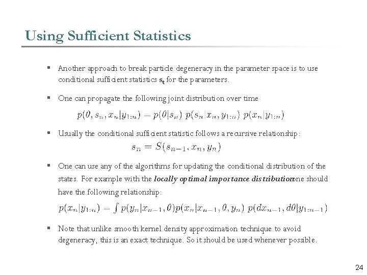
Using Sufficient Statistics § Another approach to break particle degeneracy in the parameter space is to use conditional sufficient statistics st for the parameters. § One can propagate the following joint distribution over time § Usually the conditional sufficient statistic follows a recursive relationship: § One can use any of the algorithms for updating the conditional distribution of the states. For example with the locally optimal importance distributionone should have the following relationship: § Note that unlike smooth kernel density approximation technique to avoid degeneracy, this is an exact technique. So it should be used whenever possible. 24

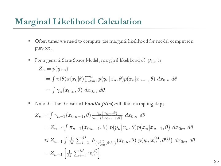
Marginal Likelihood Calculation § Often times we need to compute the marginal likelihood for model comparison purpose. § For a general State Space Model, marginal likelihood of is: § Note that for the case of Vanilla filter(with the resampling step): 25

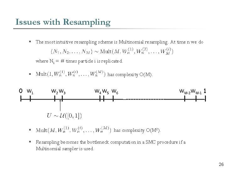
Issues with Resampling § The most intuitive resampling scheme is Multinomial resampling. At time n we do where Ni = # times particle i is replicated. § 0 W 1 § has complexity O(M). W 2 W 3 W 4 W 5 W 6 WM-2 WM-1 1 has complexity O(M 2). § Resampling becomes the bottleneck computation in a SMC procedure if a Multinomial sampler is used. 26

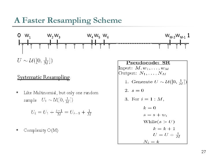
A Faster Resampling Scheme 0 W 1 W 2 W 3 W 4 W 5 W 6 WM-2 WM-1 1 Systematic Resampling: § Like Multinomial, but only one random sample § Complexity O(M) 27

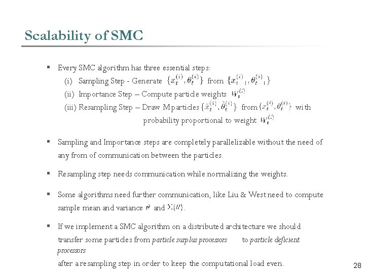
Scalability of SMC § Every SMC algorithm has three essential steps: (i) Sampling Step - Generate from (ii) Importance Step – Compute particle weights (iii) Resampling Step – Draw M particles from probability proportional to weight with § Sampling and Importance steps are completely parallelizable without the need of any from of communication between the particles. § Resampling step needs communication while normalizing the weights. § Some algorithms need further communication, like Liu & West need to compute sample mean and variance and. § If we implement a SMC algorithm on a distributed architecture we should transfer some particles from particle surplus processors to particle deficient processors after a resampling step in order to keep the computational load even. 28

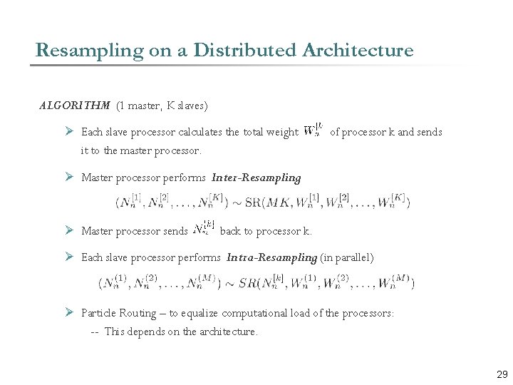
Resampling on a Distributed Architecture ALGORITHM (1 master, K slaves) Ø Each slave processor calculates the total weight it to the master processor. of processor k and sends Ø Master processor performs Inter-Resampling: Ø Master processor sends back to processor k. Ø Each slave processor performs Intra-Resampling : (in parallel) Ø Particle Routing – to equalize computational load of the processors: -- This depends on the architecture. 29

Minimal Quorum Sensing Model 30

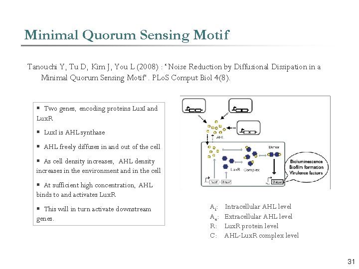
Minimal Quorum Sensing Motif Tanouchi Y, Tu D, Kim J, You L (2008) : “Noise Reduction by Diffusional Dissipation in a Minimal Quorum Sensing Motif”. PLo. S Comput Biol 4(8). § Two genes, encoding proteins Lux. I and Lux. R § Lux. I is AHL synthase § AHL freely diffuses in and out of the cell § As cell density increases, AHL density increases in the environment and in the cell § At sufficient high concentration, AHL binds to and activates Lux. R § This will in turn activate downstream genes. Ai: Ae: R: C: Intracellular AHL level Extracellular AHL level Lux. R protein level AHL-Lux. R complex level 31

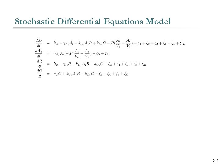
Stochastic Differential Equations Model 32

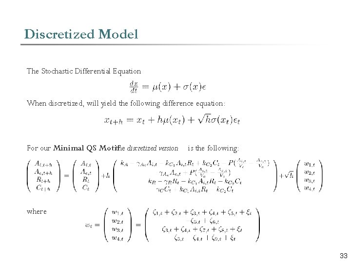
Discretized Model The Stochastic Differential Equation When discretized, will yield the following difference equation: For our Minimal QS Motif the discretized version is the following: where 33

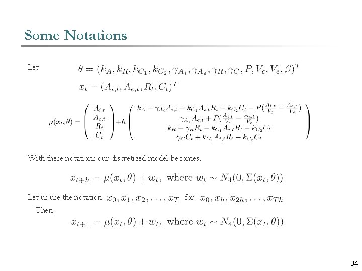
Some Notations Let With these notations our discretized model becomes: Let us use the notation Then, for 34

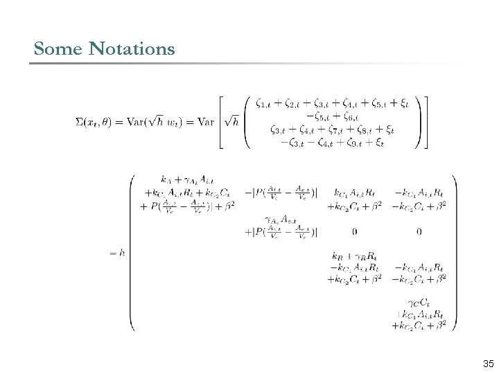
Some Notations 35

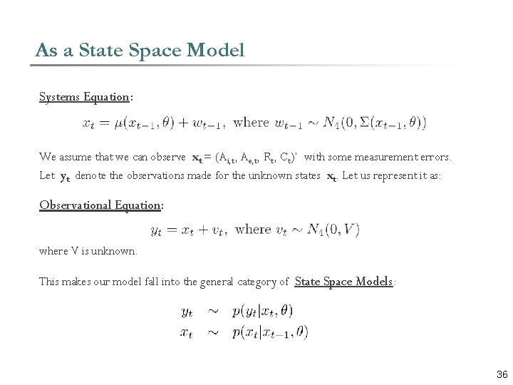
As a State Space Model Systems Equation: We assume that we can observe xt = (Ai, t, Ae, t, Rt, Ct)’ with some measurement errors. Let yt denote the observations made for the unknown states xt. Let us represent it as: Observational Equation: where V is unknown. This makes our model fall into the general category of State Space Models: 36

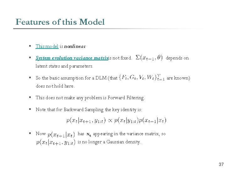
Features of this Model § This model is nonlinear. § System evolution variance matrixis not fixed. latent states and parameters. depends on § So the basic assumption for a DLM (that does not hold here. are known) § This does not make any problem is Forward Filtering. § Note that for Backward Sampling the key identity is: § Now has xt appearing in the variance matrix, so is no longer a Gaussian density. 37

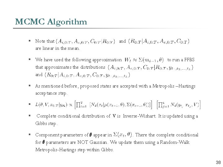
MCMC Algorithm § Note that are linear in the mean. and § We have used the following approximation that approximates the distributions and to run a FFBS § As mentioned before, proposed states are accepted with a Metropolis –Hastings acceptance step. § § Complete conditional distribution of V is Inverse-Wishart. It is updated using a Gibbs step. § Component parameters of µ appear in. There the complete conditional for µ parameters are NOT Gaussian. We update them using a Random-Walk Metropolis-Hastings step within Gibbs. 38

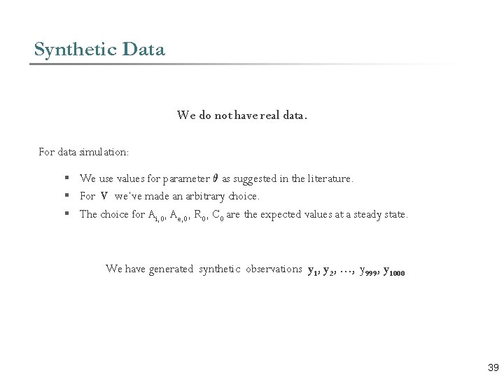
Synthetic Data We do not have real data. For data simulation: § We use values for parameter µ as suggested in the literature. § For V we’ve made an arbitrary choice. § The choice for Ai, 0, Ae, 0, R 0, C 0 are the expected values at a steady state. We have generated synthetic observations y 1, y 2, …, y 999 , y 1000 39

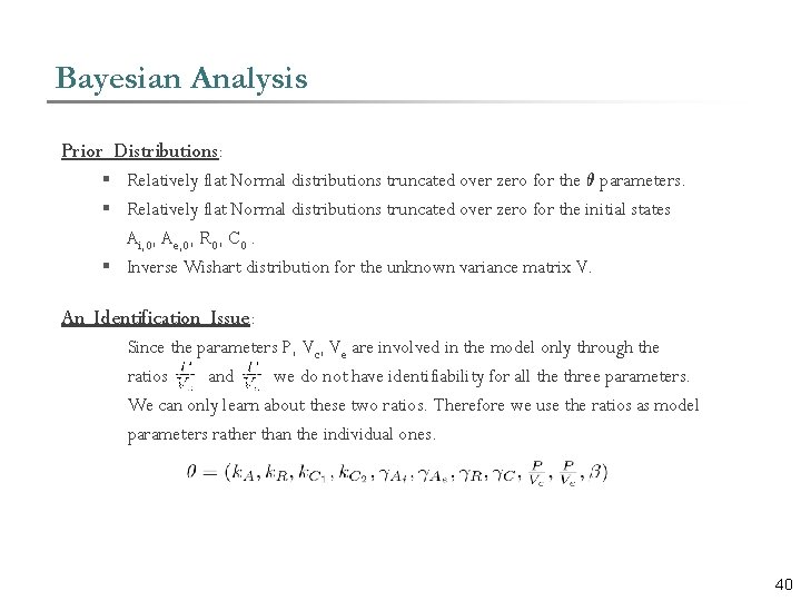
Bayesian Analysis Prior Distributions: § Relatively flat Normal distributions truncated over zero for the µ parameters. § Relatively flat Normal distributions truncated over zero for the initial states Ai, 0, Ae, 0, R 0, C 0. § Inverse Wishart distribution for the unknown variance matrix V. An Identification Issue: Since the parameters P, Vc, Ve are involved in the model only through the ratios and we do not have identifiability for all the three parameters. We can only learn about these two ratios. Therefore we use the ratios as model parameters rather than the individual ones. 40

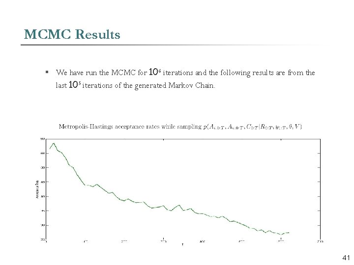
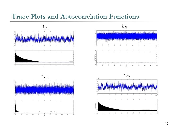
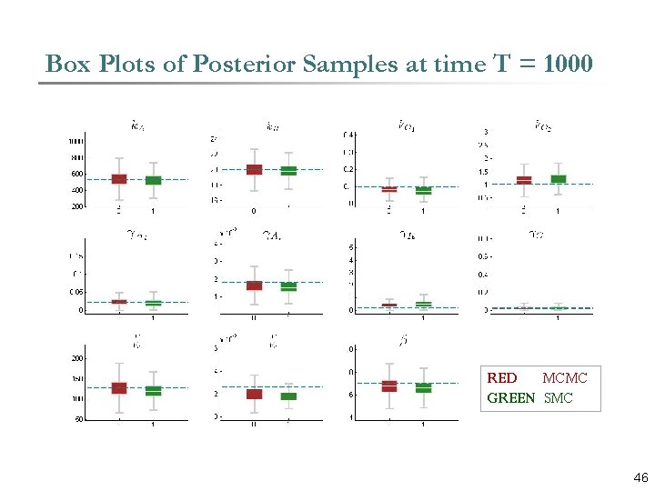
MCMC Results § We have run the MCMC for 106 iterations and the following results are from the last 105 iterations of the generated Markov Chain. 41

Trace Plots and Autocorrelation Functions 42

SMC Algorithm § We have used Auxiliary Particle Filter to reduce particle degeneracy. § For the observational equation variance matrix V, a sufficient statistics structure exists. We use the sufficient statistics to exactly sample from on each step. § For the parameters in µ no sufficient statistics structure exists. We use the kernel smoothing technique to reduce particle degeneracy in the parameter space. § We have run our particle filters with 106 particles. 43

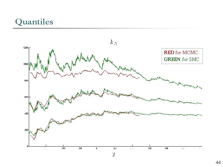
Quantiles Content RED for MCMC GREEN for SMC 44

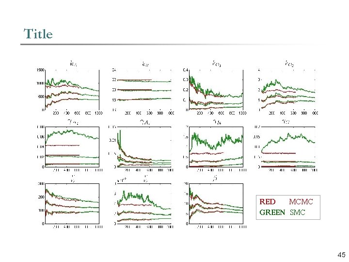
Title Content RED MCMC GREEN SMC 45

Box Plots of Posterior Samples at time T = 1000 Content RED MCMC GREEN SMC 46

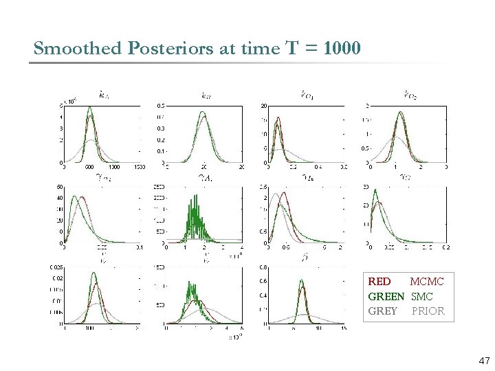
Smoothed Posteriors at time T = 1000 RED MCMC GREEN SMC GREY PRIOR 47

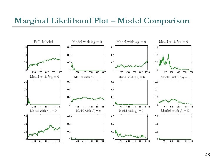
Marginal Likelihood Plot – Model Comparison Content 48

Summery § For nonlinear, non-Gaussian State space models with long time series data MCMC is slow, and has issues with convergence. § Sequential Monte Carlo techniques provide an alternative class of non-iterative algorithms to solve this class of problems. § For a long time series SMC methods suffer from degeneracy issues, particularly while computing entities like Marginal Likelihood. § SMC is scalable, so with enough resources one can imagine of tackling problems with big data which otherwise takes an enormous amount of time to solve with MCMC methods. § Model comparison becomes handy with easy computation of marginal likelihood. 49

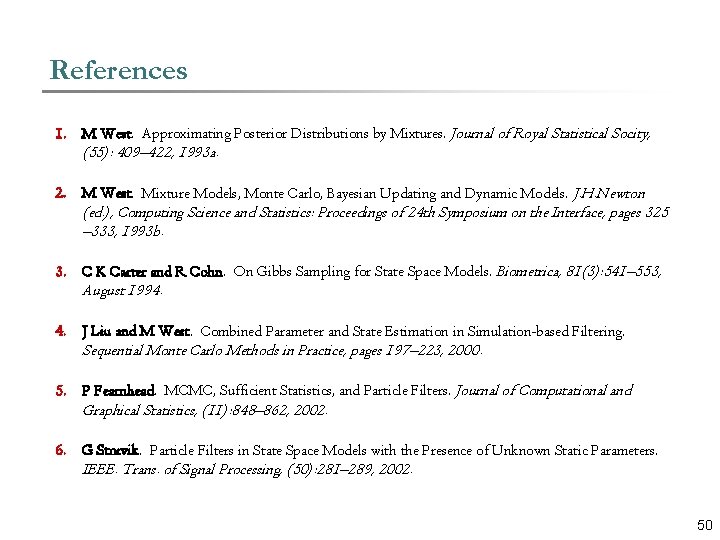
References 1. M West. Approximating Posterior Distributions by Mixtures. Journal of Royal Statistical Socity, (55): 409– 422, 1993 a. 2. M West. Mixture Models, Monte Carlo, Bayesian Updating and Dynamic Models. J. H. Newton (ed. ), Computing Science and Statistics: Proceedings of 24 th Symposium on the Interface, pages 325 – 333, 1993 b. 3. C K Carter and R Cohn. On Gibbs Sampling for State Space Models. Biometrica, 81(3): 541– 553, August 1994. 4. J Liu and M West. Combined Parameter and State Estimation in Simulation-based Filtering. Sequential Monte Carlo Methods in Practice, pages 197– 223, 2000. 5. P Fearnhead. MCMC, Sufficient Statistics, and Particle Filters. Journal of Computational and Graphical Statistics, (11): 848– 862, 2002. 6. G Storvik. Particle Filters in State Space Models with the Presence of Unknown Static Parameters. IEEE. Trans. of Signal Processing, (50): 281– 289, 2002. 50

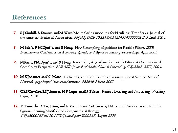
References 7. S J Godsill, A Doucet, and M West. Monte Carlo Smoothing for Nonlinear Time Series. Journal of the American Statistical Association, 99(465): DOI: 10. 1198/016214504000000151, March 2004. 8. M Boli´c, P M Djuri´c, and S Hong. New Resampling Algorithms for Particle Filters. IEEE International Conference on Acoustics, Speech, and Signal Processing, Proceedings, April 2003. 9. MBoli´c, PM Djuri´c, and S Hong. Resampling Algorithms for Particle Filters: A Computational Complexity Perspective. EURASIP Journal of Applied Signal Processing, (15): 2267– 2277, 2004. 10. M S Johannes and N Polson. Particle Filtering and Parameter Learning. Social Science Research Network, page http: //ssrn. com/abstract=983646, March 2007. 11. C M Carvalho, M Johannes, H F Lopes, and N Polson. Particle Learning and Smoothing. Working Paper, 2008. 12. Y Tanouchi, D Tu, J Kim, and L You. Noise Reduction by Diffusional Dissipation in a Minimal Quorum Sensing Motif. PLo. S Computational Biology, 4(8): e 1000167. doi: 10. 1371/journal. pcbi. 1000167, August 2008. 51

THANK YOU 52