Linear machines mrc 9 1 Decison surfaces We

Linear machines márc. 9.

1 Decison surfaces • We focus now on the decision surfaces • Linear machines = linear decision surface • Non-optimal solution but tractable model

Decision surface for Bayes classifier with Normal densites ( i = esete)

Decision tree and decision regions

Linear discriminant function two category classifier: choose 1 if g(x) > 0 else choose 2 if g(x) < 0 If g(x) = 0 the decision is undefined. g(x)=0 defines the decision surface Linear machine = linear discriminant function: g(x) = wtx + w 0 w weight vector w 0 constant bias 4

5

More than 2 categories c linear discriminant function: i is predicted if gi(x) > gj(x) j i; i. e. pairwise decision surfaces defines the decision regions 6

7

Expression power of linear machines It is proved that linear machines can only define convex regions, i. e. concave regions cannot be learnt. Moreover the decision boundaries can be higher order surfaces (like elliptoids)… 8

Homogen coordinates

10 Training linear machines

Lineáris gépek tanulása • Searching for the values of w which separates classes • Usually a goodness function is utilised as objective function, e. g. 11

Two categories - normalisation if yi belongs to ω2 replace yi by -yi then search for a which atyi>0 (normalised version) There isn’t any unique solution. 12

Iterative optimalisation • The solution minimalises J(a) • Iterative improvement of J(a) a(k+1) a(k) Step direction Learning rate 13

14 Gradient descent Learning rate is a function of k, i. e. it describes a cooling strategy

Gradient descent 15

Learning rate? 16

Perceptron rule

Perceptron szabály Y(a): the set of training samples misclassified by a If Y(a) is empty Jp(a)=0; else Jp(a)>0

Perceptron rule – Using Jp(a) in the gradient descent: 19

20 Misclassified training samples by a(k) Perceptron convergence theorem: If the training dataset is linearly separable the batch perceptron algorithm finds a solution in finete steps.

21 η(k)=1 online learning Stochastic gradient desent: Estimate the gradient based on a few trainging examples

Online vs offline learning Online learning algorithms: The modell is updated by each training instance (or by a small batch) Offline learning algorithms: The training dataset is processed as a whole Advantages of online learning: - Update is straightforward - The training dataset can be streamed - Implicit adaptation Disadvantages of online learning: - Its accuracy migth be lower

23 Not linearly separable case – Change the loss function, it should count each training example e. g. the directed distance from the decision surface

SVM

25 Which one to prefer?

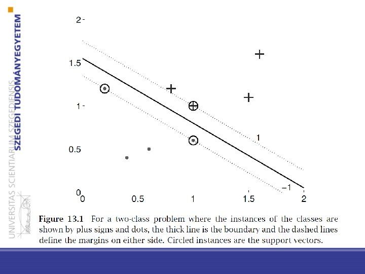
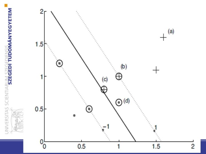
26 • Margin: the gap around the decision surface. It is defined by the training instances closest to the decision survey (support vectors)

27

Support Vector Machine (SVM) 28 • SVM is a linear machine where the objective function incorporates the maximalisation of the margin! • This provides generalisation ability •

SVM Linearly separable case

Linear SVM: linearly separable case • Training database: • Searching for w s. t. or 30

Linear SVM: linearly separable case • Note the size of the margin by ρ • Linearly separable: • We prefer a unique solution: • argmax ρ = argmin 31

Linear SVM: linearly separable case 32 Convex quadratic optimisation problem…

Linear SVM: linearly separable case The form of the solution: Weighted avearge of training instances bármely t-ből xt támasztóvektor iff only support vectors count 33

SVM not linearly separable case

• ξ slack variable enables incorrect classifications („soft margin”): ξt=0 if the classification is correct, else it is the distance from the margin C is a metaparameter for the trade-off between the margin size and incorrect classifications Linear SVM: not linearly separable case 36

SVM non-linear case

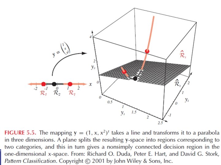
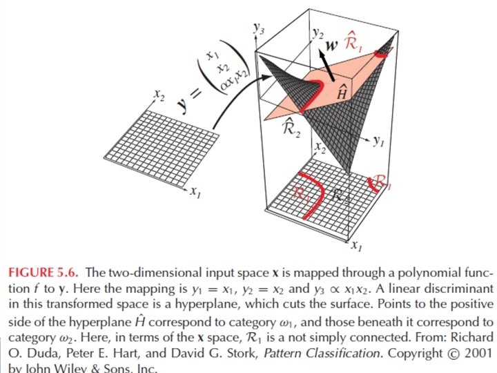
Generalised linear discriminant functions • E. g. quadratic decision surface: • Generalised linear discriminant functions: yi: Rd → R arbitrary functions g(x) is not linear in x, but is is linear in yi (it is a hyperplane in the y-space)

Example

Non-linear SVM 43

Non-linear SVM Φ is a mapping into a higher dimensional (k) space: There exists a mapping into a higher dimensional space for any dataset where the dataset will be linearly separable in the new space. 44

The kernel trick g(x)= The calculation of mappings into high dimensional space can be omited if the kernel of to x can be computed 45

46 Example: polinomial kernel K(x, y)=(x y) p d=256 (original dimensions) p=4 h=183 181 376 (high dimensional space) on the other hand K(x, y) is known and feasible to calculate while the inner product in high dimensions is not

47 Kernels in practice • No rule of thumbs for selecting the appropiate kernel

48 The XOR example

49 The XOR example

50 The XOR example

51 The XOR example

52 Notes on SVM • Training is a global optimalisation problem (exact optimalisation). • The performance of SVM is highly dependent on the choice of the kernel and its parameters • Finding the appropriate kernel for a particular task is „magic”

53 Notes on SVM • Complexity depends on the number of support vectors but not on the dimensionality of the feature space • In practice, it gaines good enogh generalisation ability even with a small training database

Summary • • Linear machines Gradient descent Perceptron SVM – Linearly separable case – Not separable case – Non-linear SVM