Lecture 9 Sequential Networks Implementation CSE 140 Components

Lecture 9: Sequential Networks: Implementation CSE 140: Components and Design Techniques for Digital Systems Fall 2014 CK Cheng Dept. of Computer Science and Engineering University of California, San Diego 1

Implementation • • Format and Tool Procedure Excitation Tables Example 2

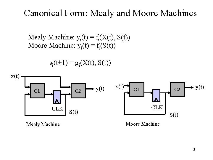
Canonical Form: Mealy and Moore Machines Mealy Machine: yi(t) = fi(X(t), S(t)) Moore Machine: yi(t) = fi(S(t)) si(t+1) = gi(X(t), S(t)) x(t) C 1 C 2 CLK Mealy Machine S(t) y(t) x(t) C 1 y(t) C 2 CLK S(t) Moore Machine 3

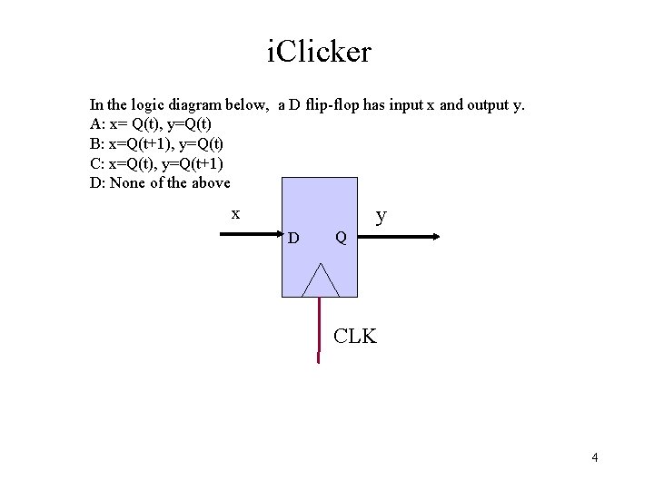
i. Clicker In the logic diagram below, a D flip-flop has input x and output y. A: x= Q(t), y=Q(t) B: x=Q(t+1), y=Q(t) C: x=Q(t), y=Q(t+1) D: None of the above y x D Q CLK 4

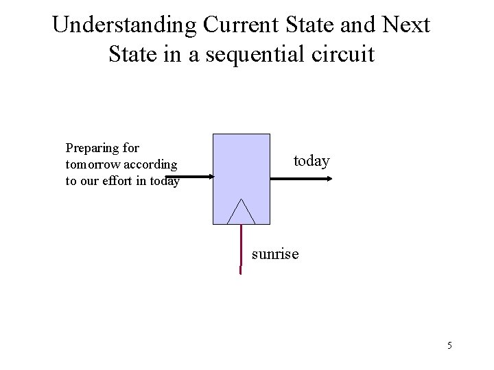
Understanding Current State and Next State in a sequential circuit Preparing for tomorrow according to our effort in today sunrise 5

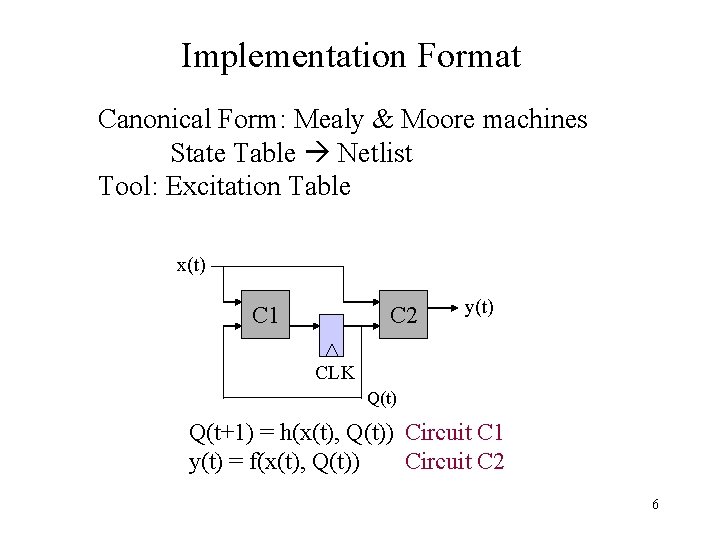
Implementation Format Canonical Form: Mealy & Moore machines State Table Netlist Tool: Excitation Table x(t) C 1 C 2 y(t) CLK Q(t) Q(t+1) = h(x(t), Q(t)) Circuit C 1 y(t) = f(x(t), Q(t)) Circuit C 2 6

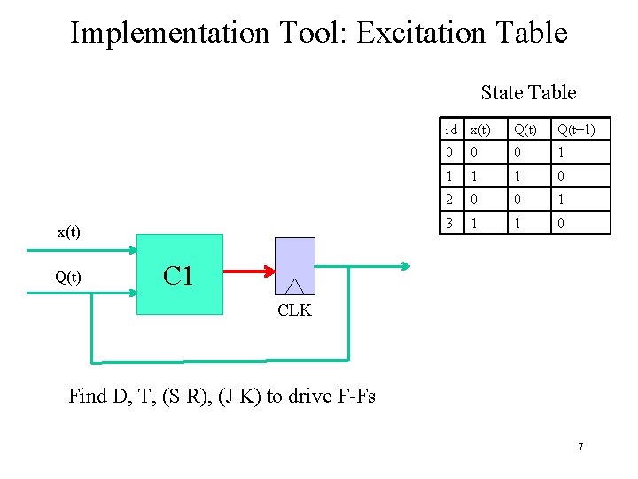
Implementation Tool: Excitation Table State Table x(t) Q(t) id x(t) Q(t+1) 0 0 0 1 1 0 2 0 0 1 3 1 1 0 C 1 CLK Find D, T, (S R), (J K) to drive F-Fs 7

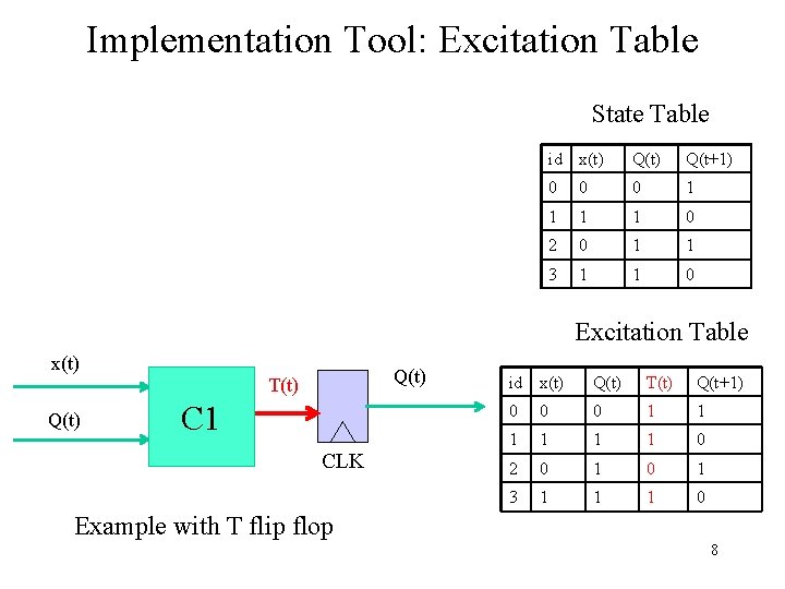
Implementation Tool: Excitation Table State Table id x(t) Q(t+1) 0 0 0 1 1 0 2 0 1 1 3 1 1 0 Excitation Table x(t) Q(t) T(t) Q(t) C 1 CLK id x(t) Q(t) T(t) Q(t+1) 0 0 0 1 1 1 0 2 0 1 3 1 1 1 0 Example with T flip flop 8

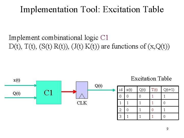
Implementation Tool: Excitation Table Implement combinational logic C 1 D(t), T(t), (S(t) R(t)), (J(t) K(t)) are functions of (x, Q(t)) Excitation Table x(t) Q(t) C 1 CLK id x(t) Q(t) T(t) Q(t+1) 0 0 0 1 1 1 0 2 0 1 3 1 1 1 0 9

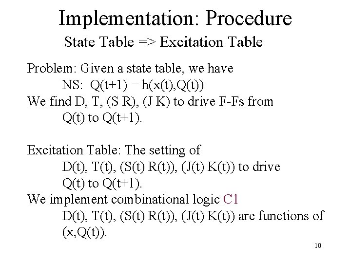
Implementation: Procedure State Table => Excitation Table Problem: Given a state table, we have NS: Q(t+1) = h(x(t), Q(t)) We find D, T, (S R), (J K) to drive F-Fs from Q(t) to Q(t+1). Excitation Table: The setting of D(t), T(t), (S(t) R(t)), (J(t) K(t)) to drive Q(t) to Q(t+1). We implement combinational logic C 1 D(t), T(t), (S(t) R(t)), (J(t) K(t)) are functions of (x, Q(t)). 10

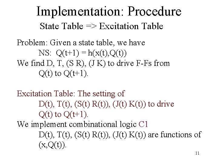
Implementation: Procedure State Table => Excitation Table Problem: Given a state table, we have NS: Q(t+1) = h(x(t), Q(t)) We find D, T, (S R), (J K) to drive F-Fs from Q(t) to Q(t+1). Excitation Table: The setting of D(t), T(t), (S(t) R(t)), (J(t) K(t)) to drive Q(t) to Q(t+1). We implement combinational logic C 1 D(t), T(t), (S(t) R(t)), (J(t) K(t)) are functions of (x, Q(t)). 11

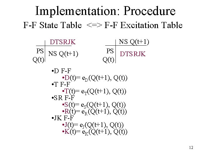
Implementation: Procedure F-F State Table <=> F-F Excitation Table DTSRJK PS NS Q(t+1) Q(t) NS Q(t+1) PS DTSRJK Q(t) • D F-F • D(t)= e. D(Q(t+1), Q(t)) • T F-F • T(t)= e. T(Q(t+1), Q(t)) • SR F-F • S(t)= e. S(Q(t+1), Q(t)) • R(t)= e. R(Q(t+1), Q(t)) • JK F-F • J(t)= e. J(Q(t+1), Q(t)) • K(t)= e. K(Q(t+1), Q(t)) 12

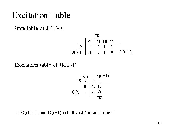
Excitation Table State table of JK F-F: JK 00 01 10 11 0 0 1 1 1 0 0 Q(t) 1 Q(t+1) Excitation table of JK F-F: PS Q(t) NS 0 1 Q(t+1) 0 1 0 - 1 -1 -0 JK If Q(t) is 1, and Q(t+1) is 0, then JK needs to be -1. 13

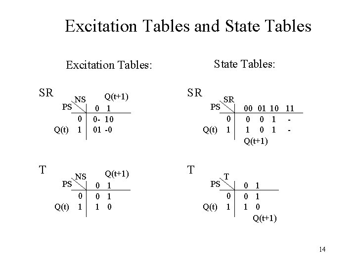
Excitation Tables and State Tables: Excitation Tables: SR PS Q(t) T PS Q(t) NS 0 1 Q(t+1) 0 1 0 - 10 01 -0 Q(t+1) 0 1 1 0 SR PS Q(t) T PS Q(t) SR 0 1 T 0 1 00 01 10 11 0 0 1 1 0 1 Q(t+1) 0 1 1 0 Q(t+1) 14

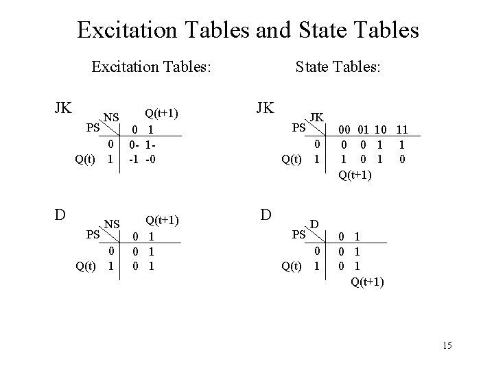
Excitation Tables and State Tables Excitation Tables: JK PS Q(t) D PS Q(t) NS 0 1 Q(t+1) 0 1 0 - 1 -1 -0 Q(t+1) 0 1 0 1 State Tables: JK PS Q(t) D PS Q(t) JK 0 1 D 0 1 00 01 10 11 0 0 1 1 1 0 Q(t+1) 0 1 0 1 Q(t+1) 15

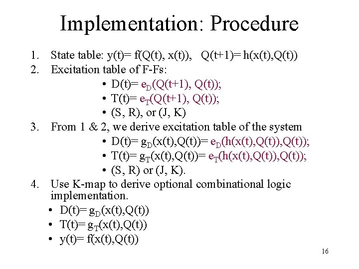
Implementation: Procedure 1. State table: y(t)= f(Q(t), x(t)), Q(t+1)= h(x(t), Q(t)) 2. Excitation table of F-Fs: • D(t)= e. D(Q(t+1), Q(t)); • T(t)= e. T(Q(t+1), Q(t)); • (S, R), or (J, K) 3. From 1 & 2, we derive excitation table of the system • D(t)= g. D(x(t), Q(t))= e. D(h(x(t), Q(t)); • T(t)= g. T(x(t), Q(t))= e. T(h(x(t), Q(t)); • (S, R) or (J, K). 4. Use K-map to derive optional combinational logic implementation. • D(t)= g. D(x(t), Q(t)) • T(t)= g. T(x(t), Q(t)) • y(t)= f(x(t), Q(t)) 16

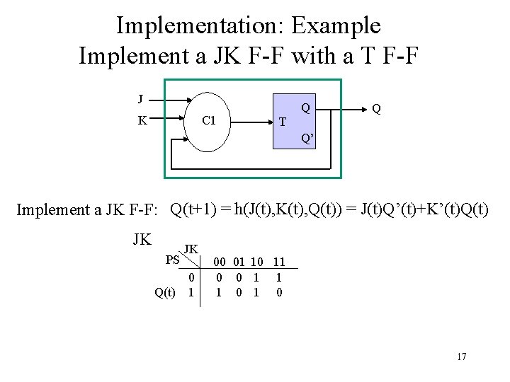
Implementation: Example Implement a JK F-F with a T F-F J K C 1 T Q Q Q’ Implement a JK F-F: Q(t+1) = h(J(t), K(t), Q(t)) = J(t)Q’(t)+K’(t)Q(t) JK PS Q(t) JK 0 1 00 01 10 11 0 0 1 1 1 0 17

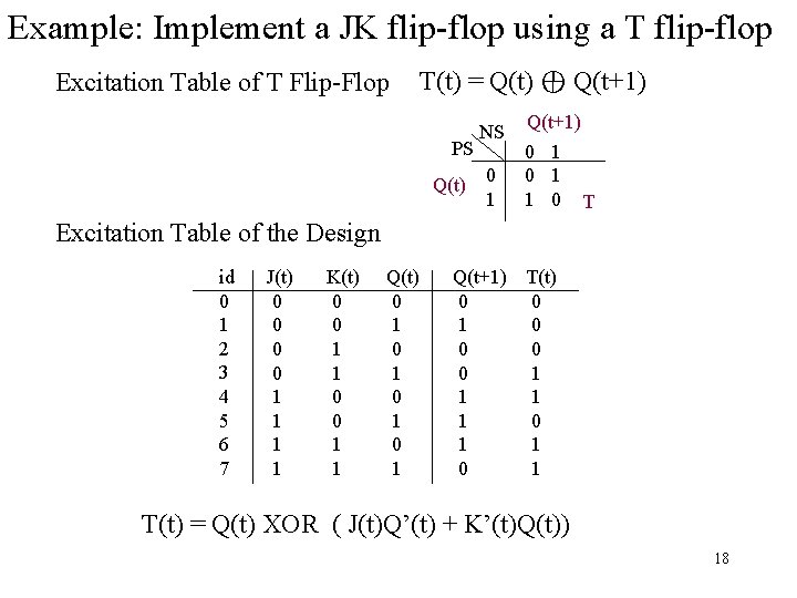
Example: Implement a JK flip-flop using a T flip-flop Excitation Table of T Flip-Flop T(t) = Q(t) ⊕ Q(t+1) PS Q(t) NS 0 1 Q(t+1) 0 1 1 0 T Excitation Table of the Design id 0 1 2 3 4 5 6 7 J(t) 0 0 1 1 K(t) 0 0 1 1 Q(t) 0 1 0 1 Q(t+1) T(t) 0 0 1 1 0 1 T(t) = Q(t) XOR ( J(t)Q’(t) + K’(t)Q(t)) 18

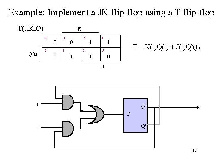
Example: Implement a JK flip-flop using a T flip-flop T(J, K, Q): 0 Q(t) K 0 1 2 0 3 0 6 1 7 1 4 1 T = K(t)Q(t) + J(t)Q’(t) 5 1 0 J J Q T K Q’ 19

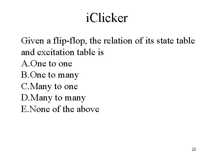
i. Clicker Given a flip-flop, the relation of its state table and excitation table is A. One to one B. One to many C. Many to one D. Many to many E. None of the above 20

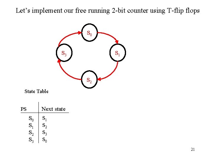
Let’s implement our free running 2 -bit counter using T-flip flops S 0 S 1 S 3 S 2 State Table Next state PS S 0 S 1 S 2 S 3 S 0 21

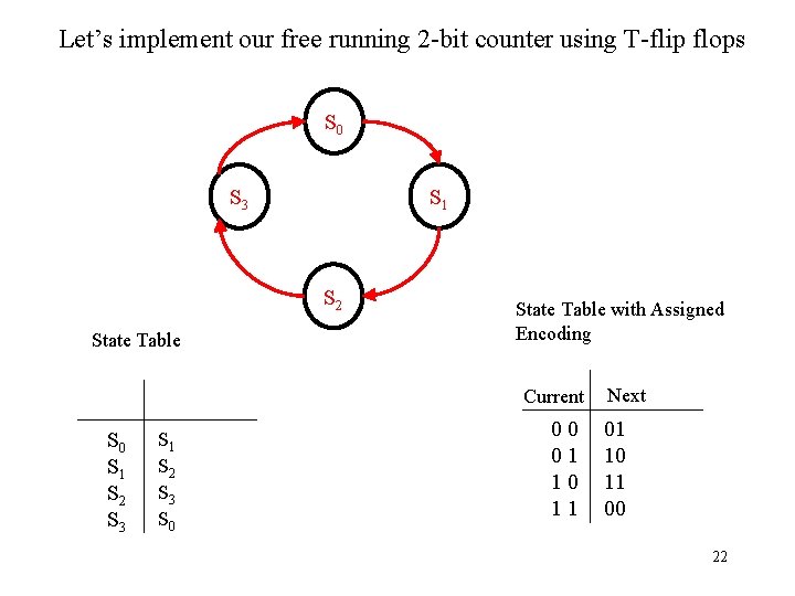
Let’s implement our free running 2 -bit counter using T-flip flops S 0 S 1 S 3 S 2 State Table with Assigned Encoding Current S 0 S 1 S 2 S 3 S 0 00 01 10 11 Next 01 10 11 00 22

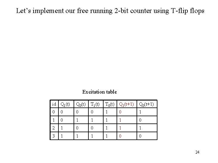
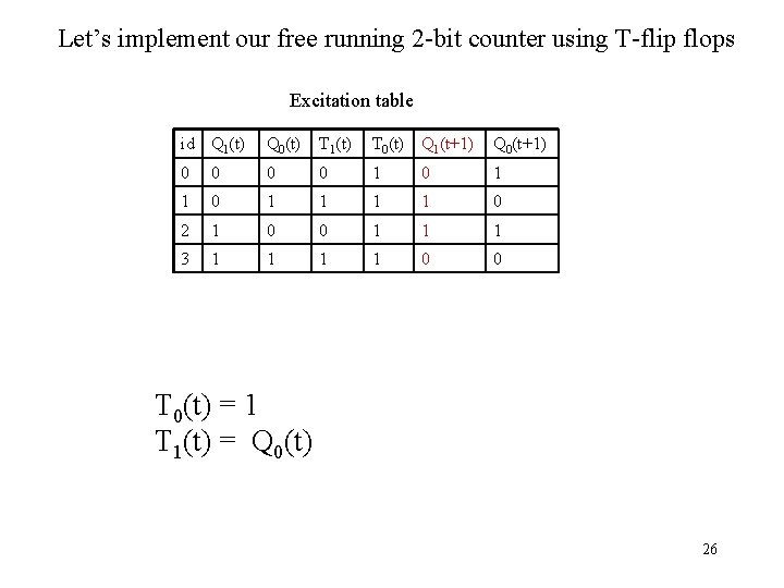
Let’s implement our free running 2 -bit counter using T-flip flops Excitation table id Q 1(t) Q 0(t) T 1(t) T 0(t) Q 1(t+1) Q 0(t+1) 0 0 1 1 0 2 1 0 1 1 3 1 1 0 0 23

Let’s implement our free running 2 -bit counter using T-flip flops Excitation table id Q 1(t) Q 0(t) T 1(t) T 0(t) Q 1(t+1) Q 0(t+1) 0 0 1 0 1 1 1 1 0 2 1 0 0 1 1 1 3 1 1 0 0 24

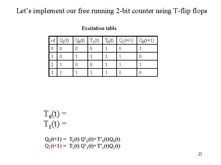
Let’s implement our free running 2 -bit counter using T-flip flops Excitation table id Q 1(t) Q 0(t) T 1(t) T 0(t) Q 1(t+1) Q 0(t+1) 0 0 1 0 1 1 1 1 0 2 1 0 0 1 1 1 3 1 1 0 0 T 0(t) = T 1(t) = Q 0(t+1) = T 0(t) Q’ 0(t)+T’ 0(t)Q 0(t) Q 1(t+1) = T 1(t) Q’ 1(t)+T’ 1(t)Q 1(t) 25

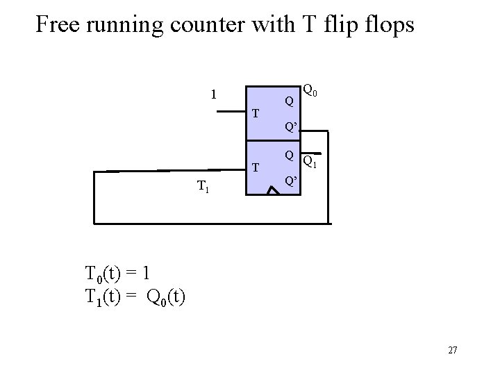
Let’s implement our free running 2 -bit counter using T-flip flops Excitation table id Q 1(t) Q 0(t) T 1(t) T 0(t) Q 1(t+1) Q 0(t+1) 0 0 1 0 1 1 1 1 0 2 1 0 0 1 1 1 3 1 1 0 0 T 0(t) = 1 T 1(t) = Q 0(t) 26

Free running counter with T flip flops 1 T T T 1 Q Q 0 Q’ Q Q 1 Q’ T 0(t) = 1 T 1(t) = Q 0(t) 27

Implementation: State Diagram => State Table => Netlist Pattern Recognizer: A sequential machine has a binary input x in {a, b}. For x(t-2, t) = aab, the output y(t) = 1, otherwise y(t) = 0. Assign mapping a: 0, b: 1 28

Implementation: State Diagram => State Table => Netlist Pattern Recognizer: A sequential machine has a binary input x in {a, b}. For x(t-2, t) = aab, the output y(t) = 1, otherwise y(t) = 0. Assign mapping a: 0, b: 1 PI Q How many states should the pattern recognizer have A. One because it has one output B. One because it has one input C. Two because the input can be one of two states (a or b) D. Three because. . . . E. Four because. . . 29

PI Q: How many states should the pattern recognizer have A. One because it has one output B. One because it has one input C. Two because the input can be one of two states (a or b) D. Three because. . . . E. Four because. . . 30

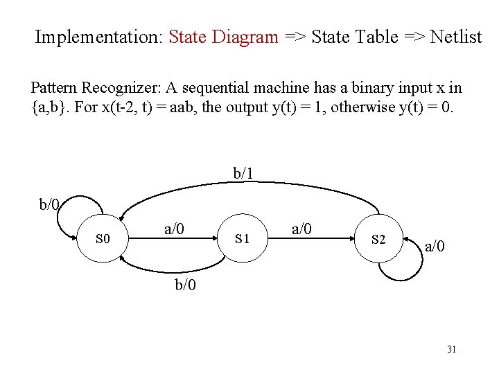
Implementation: State Diagram => State Table => Netlist Pattern Recognizer: A sequential machine has a binary input x in {a, b}. For x(t-2, t) = aab, the output y(t) = 1, otherwise y(t) = 0. b/1 b/0 S 0 a/0 S 1 a/0 S 2 a/0 b/0 31

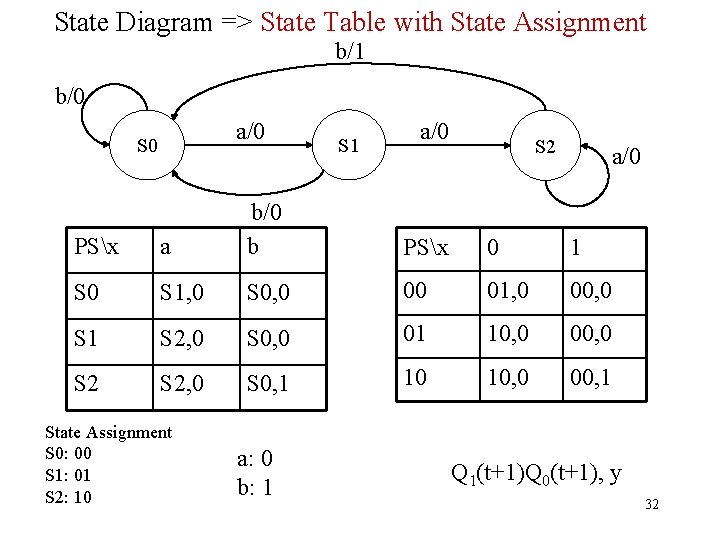
State Diagram => State Table with State Assignment b/1 b/0 a/0 S 1 a/0 S 2 a/0 PSx a b/0 b S 0 S 1, 0 S 0, 0 00 01, 0 00, 0 S 1 S 2, 0 S 0, 0 01 10, 0 00, 0 S 2, 0 S 0, 1 10 10, 0 00, 1 State Assignment S 0: 00 S 1: 01 S 2: 10 a: 0 b: 1 PSx 0 1 Q 1(t+1)Q 0(t+1), y 32

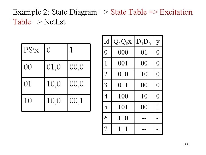
Example 2: State Diagram => State Table => Excitation Table => Netlist PSx 0 1 00 01, 0 01 10, 0 10 10, 0 id Q 1 Q 0 x D 1 D 0 y 0 000 01 0 00, 0 1 00 0 2 010 10 0 00, 0 3 011 00 0 4 100 10 0 5 101 00 1 6 110 -- - 7 111 -- - 00, 1 33

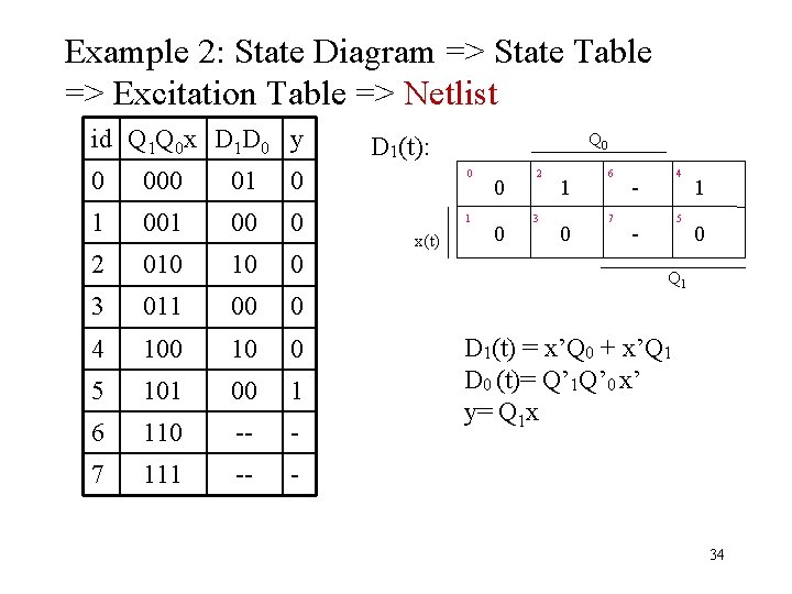
Example 2: State Diagram => State Table => Excitation Table => Netlist id Q 1 Q 0 x D 1 D 0 y Q 0 D 1(t): 0 000 01 0 0 1 00 0 1 2 010 10 0 3 011 00 0 4 100 10 0 5 101 00 1 6 110 -- - 7 111 -- - x(t) 0 0 2 3 1 0 6 7 4 - 5 - 1 0 Q 1 D 1(t) = x’Q 0 + x’Q 1 D 0 (t)= Q’ 1 Q’ 0 x’ y= Q 1 x 34

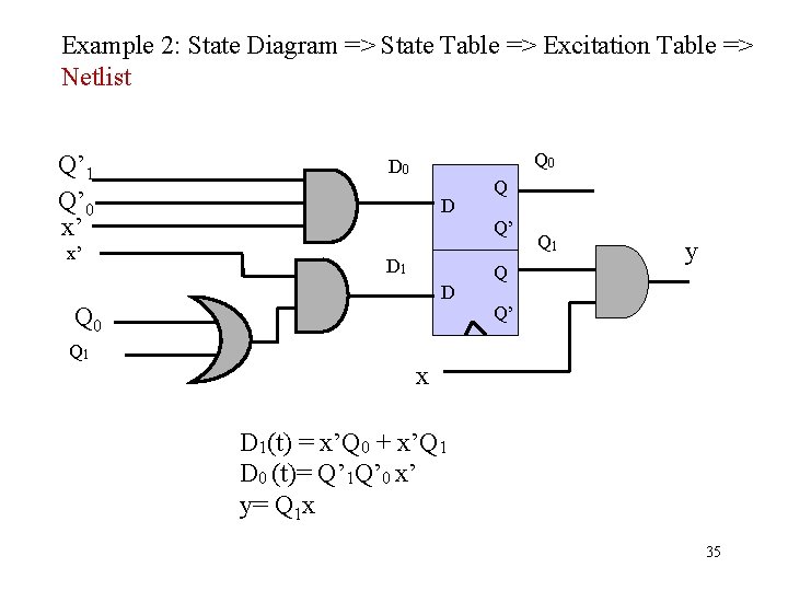
Example 2: State Diagram => State Table => Excitation Table => Netlist Q’ 1 Q’ 0 x’ x’ Q 0 D D 1 D Q 0 Q 1 Q Q’ Q Q 1 y Q’ x D 1(t) = x’Q 0 + x’Q 1 D 0 (t)= Q’ 1 Q’ 0 x’ y= Q 1 x 35

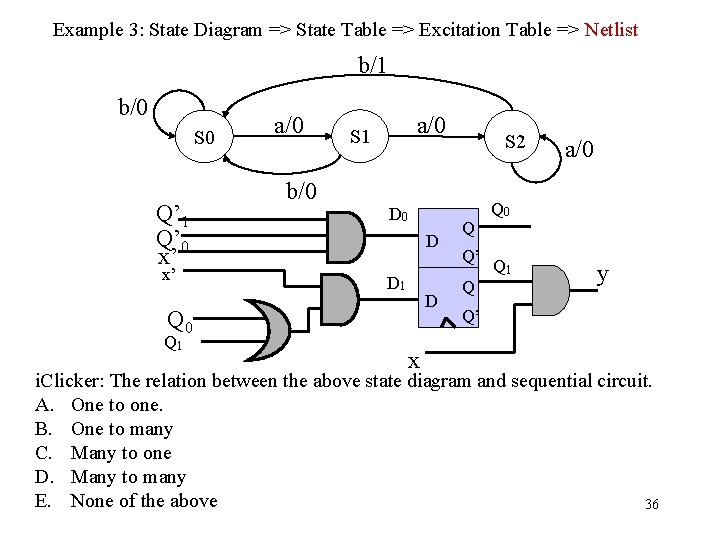
Example 3: State Diagram => State Table => Excitation Table => Netlist b/1 b/0 S 0 Q’ 1 Q’ 0 x’ x’ a/0 b/0 a/0 S 1 D 0 D D 1 D Q 0 Q 1 x S 2 Q Q’ Q a/0 Q 1 y Q’ i. Clicker: The relation between the above state diagram and sequential circuit. A. One to one. B. One to many C. Many to one D. Many to many E. None of the above 36

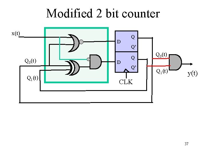
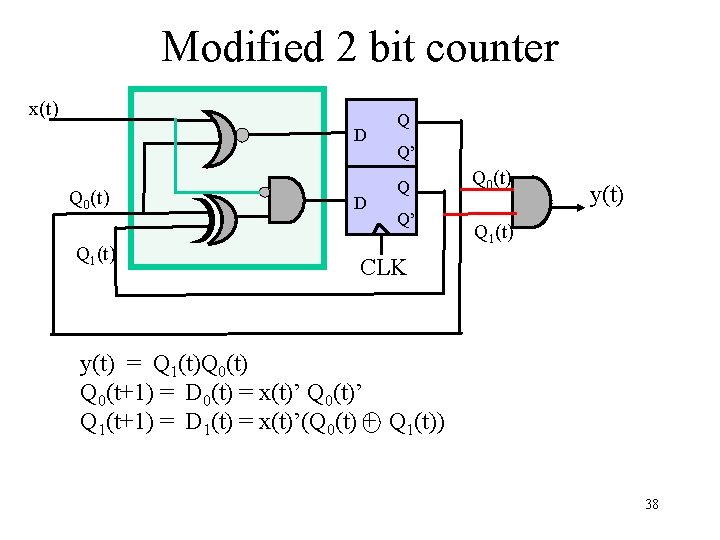
Modified 2 bit counter x(t) D Q 0(t) Q 1(t) D Q Q’ Q 0(t) Q 1(t) y(t) CLK 37

Modified 2 bit counter x(t) D Q 0(t) Q 1(t) D Q Q’ Q 0(t) y(t) Q 1(t) CLK y(t) = Q 1(t)Q 0(t) Q 0(t+1) = D 0(t) = x(t)’ Q 0(t)’ Q 1(t+1) = D 1(t) = x(t)’(Q 0(t) + Q 1(t)) 38

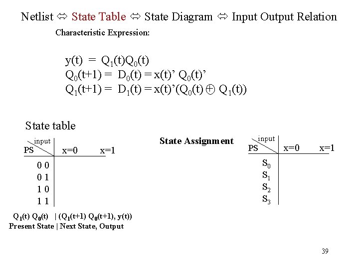
Netlist State Table State Diagram Input Output Relation Characteristic Expression: y(t) = Q 1(t)Q 0(t) Q 0(t+1) = D 0(t) = x(t)’ Q 0(t)’ Q 1(t+1) = D 1(t) = x(t)’(Q 0(t) + Q 1(t)) State table PS input x=0 x=1 00 01 10 11 State Assignment input PS x=0 x=1 S 0 S 1 S 2 S 3 Q 1(t) Q 0(t) | (Q 1(t+1) Q 0(t+1), y(t)) Present State | Next State, Output 39

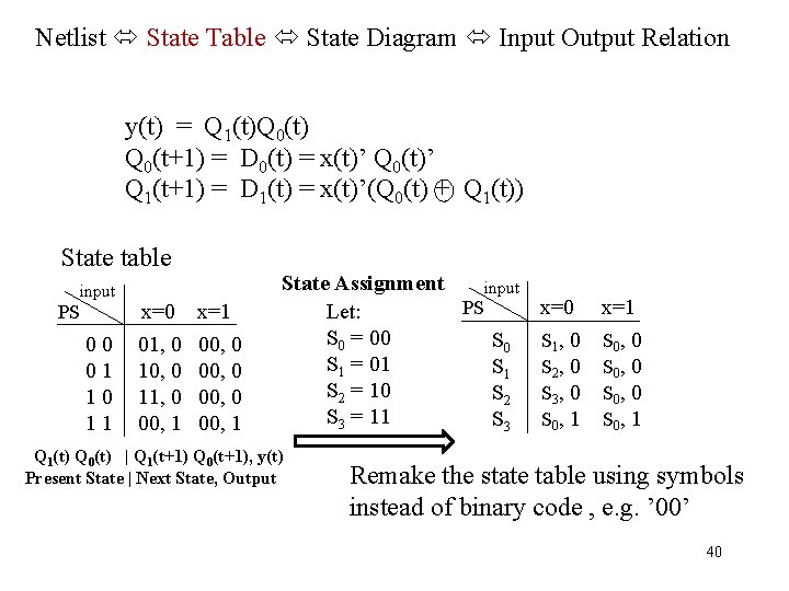
Netlist State Table State Diagram Input Output Relation y(t) = Q 1(t)Q 0(t) Q 0(t+1) = D 0(t) = x(t)’ Q 0(t)’ Q 1(t+1) = D 1(t) = x(t)’(Q 0(t) + Q 1(t)) State table PS input 00 01 10 11 x=0 01, 0 10, 0 11, 0 00, 1 x=1 00, 0 00, 1 State Assignment input PS Let: S 0 = 00 S 1 = 01 S 2 = 10 S 2 S 3 = 11 S 3 Q 1(t) Q 0(t) | Q 1(t+1) Q 0(t+1), y(t) Present State | Next State, Output x=0 S 1 , 0 S 2 , 0 S 3 , 0 S 0 , 1 x=1 S 0 , 0 S 0 , 1 Remake the state table using symbols instead of binary code , e. g. ’ 00’ 40

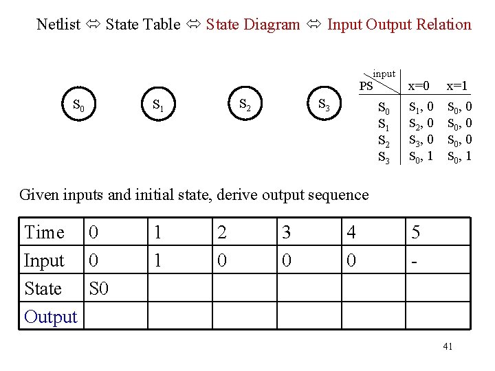
Netlist State Table State Diagram Input Output Relation input PS S 0 S 2 S 1 S 3 S 0 S 1 S 2 S 3 x=0 S 1 , 0 S 2 , 0 S 3 , 0 S 0 , 1 x=1 S 0 , 0 S 0 , 1 Given inputs and initial state, derive output sequence Time 0 Input 0 State S 0 Output 1 1 2 0 3 0 4 0 5 - 41

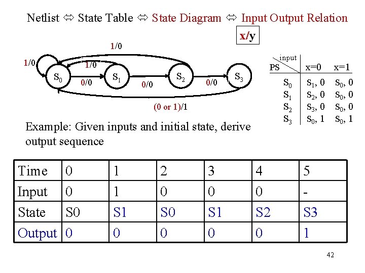
Netlist State Table State Diagram Input Output Relation x/y 1/0 input 1/0 S 0 0/0 S 1 S 2 0/0 S 3 PS S 0 S 1 S 2 S 3 (0 or 1)/1 Example: Given inputs and initial state, derive output sequence Time Input State Output 0 0 S 0 0 1 1 S 1 0 2 0 S 0 0 3 0 S 1 0 4 0 S 2 0 x=0 S 1 , 0 S 2 , 0 S 3 , 0 S 0 , 1 x=1 S 0 , 0 S 0 , 1 5 S 3 1 42

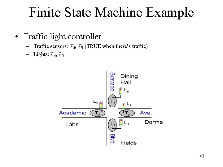
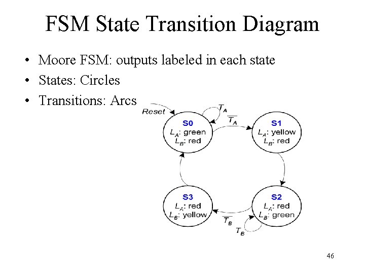
Finite State Machine Example • Traffic light controller – Traffic sensors: TA, TB (TRUE when there’s traffic) – Lights: LA, LB 43

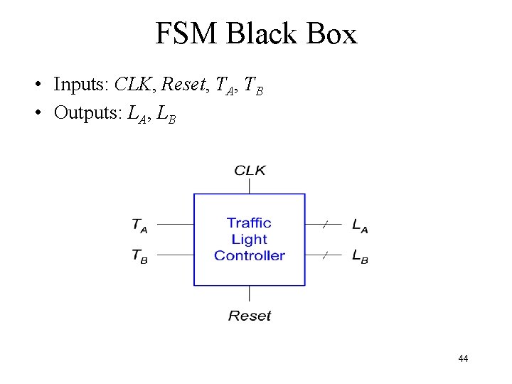
FSM Black Box • Inputs: CLK, Reset, TA, TB • Outputs: LA, LB 44

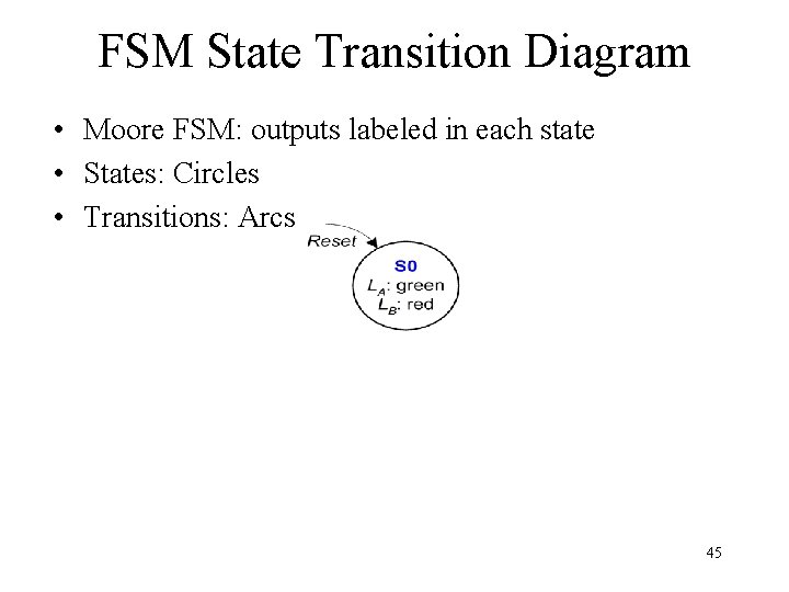
FSM State Transition Diagram • Moore FSM: outputs labeled in each state • States: Circles • Transitions: Arcs 45

FSM State Transition Diagram • Moore FSM: outputs labeled in each state • States: Circles • Transitions: Arcs 46

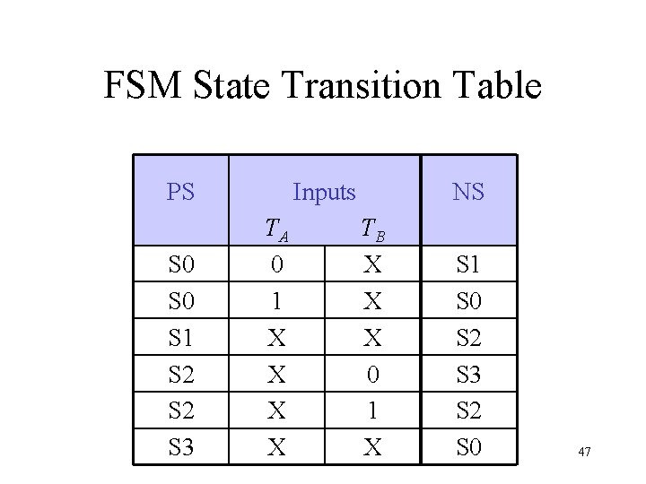
FSM State Transition Table PS S 0 S 1 S 2 S 3 Inputs TA 0 1 X X NS TB X X X 0 1 X S 1 S 0 S 2 S 3 S 2 S 0 47

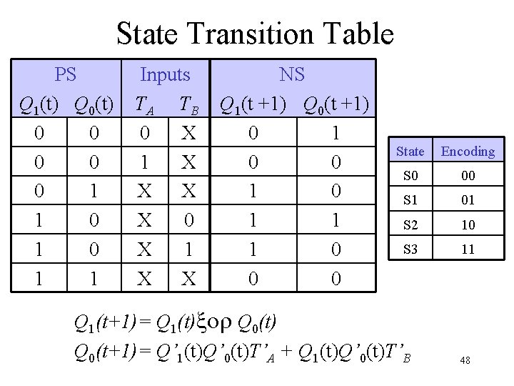
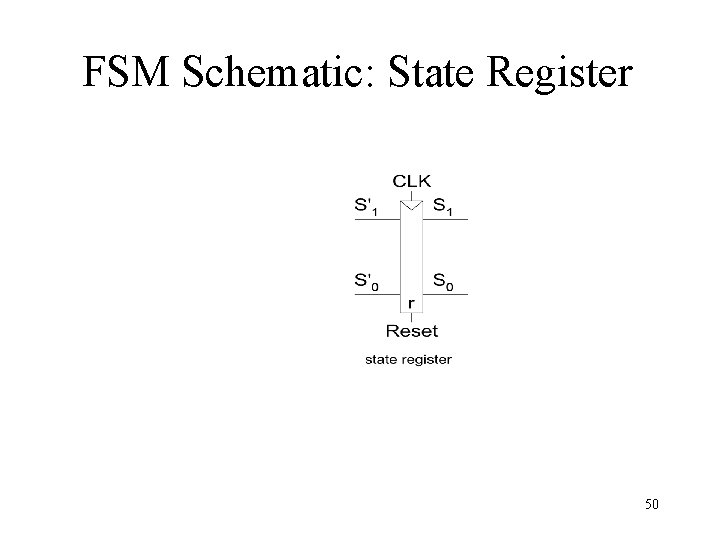
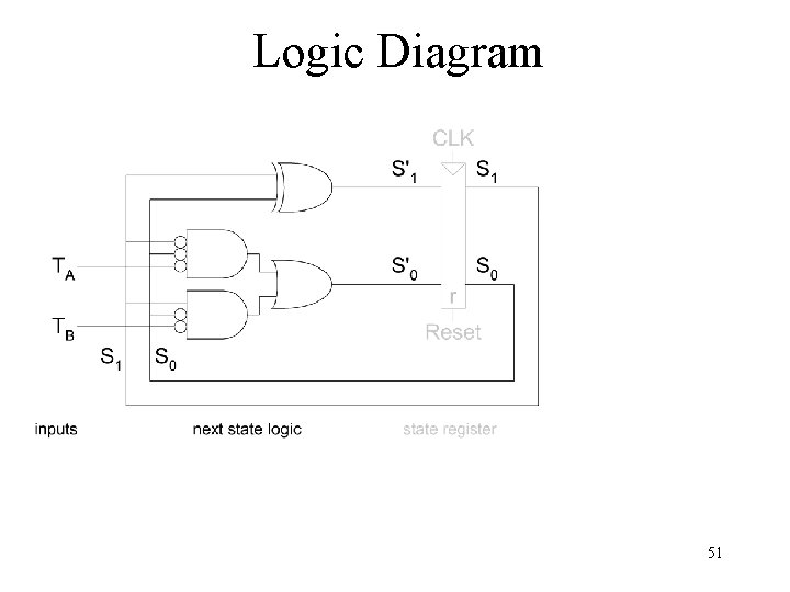
State Transition Table PS Q 1(t) Q 0(t) 0 0 0 1 1 Inputs TA TB 0 X 1 X X NS Q 1(t +1) Q 0(t +1) 0 1 0 1 1 1 0 0 0 State Encoding S 0 00 S 1 01 S 2 10 S 3 11 Q 1(t+1)= Q 1(t)xor Q 0(t) Q 0(t+1)= Q’ 1(t)Q’ 0(t)T’A + Q 1(t)Q’ 0(t)T’B 48

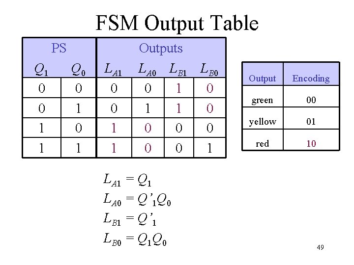
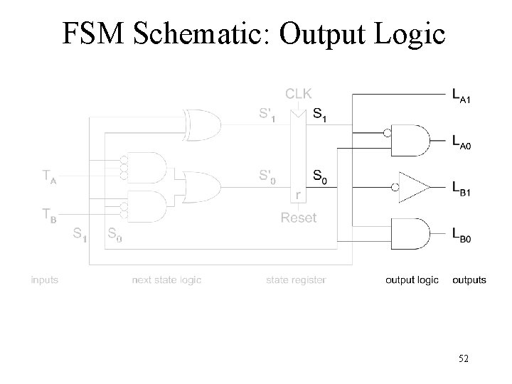
FSM Output Table PS Q 1 0 0 1 1 Q 0 0 1 LA 1 0 0 1 1 Outputs LA 0 LB 1 LB 0 0 1 1 0 0 0 1 LA 1 = Q 1 LA 0 = Q’ 1 Q 0 LB 1 = Q’ 1 LB 0 = Q 1 Q 0 Output Encoding green 00 yellow 01 red 10 49

FSM Schematic: State Register 50

Logic Diagram 51

FSM Schematic: Output Logic 52

Summary: Implementation • Set up canonical form • Mealy or Moore machine • Identify the next states • state diagram ⇨ state table • state assignment • Derive excitation table • Inputs of flip flops • Design the combinational logic • don’t care set utilization 53