Generic Rounding Schemes for SDP Relaxations Prasad Raghavendra

Generic Rounding Schemes for SDP Relaxations Prasad Raghavendra Georgia Institute of Technology, Atlanta

``Squish and Solve” Rounding Schemes [R, Steurer 2009] Rounding Schemes via Dictatorship Tests [R, 2008] Rounding SDP Hierarchies via Correlation [Barak, R, Steurer 2011] [R, Tan 2011]

``Squish and Solve” Rounding Schemes [R, Steurer 2009]

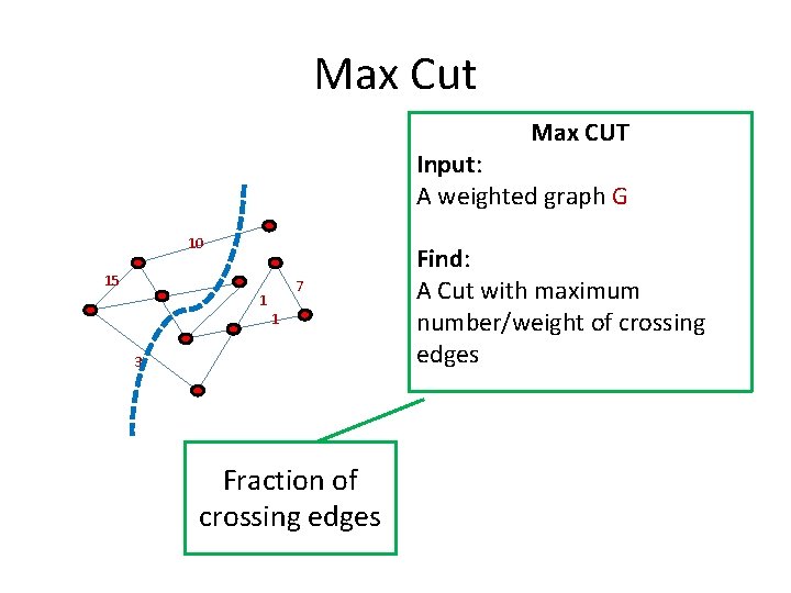
Max Cut Max CUT Input: A weighted graph G 10 15 7 1 1 3 Fraction of crossing edges Find: A Cut with maximum number/weight of crossing edges

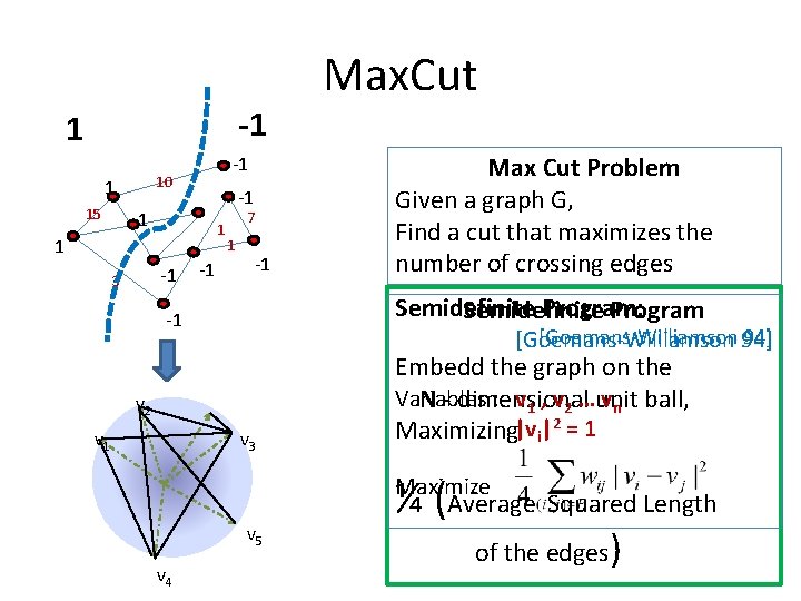
-1 1 10 1 15 -1 -1 3 -1 7 1 -1 Max Cut Problem Given a graph G, Find a cut that maximizes the number of crossing edges Semidefinite Program: Semidefinite Program -1 [Goemans-Williamson 94] [Goemans-Williamson v 2 v 1 Max. Cut v 3 Embedd the graph on the Variables : v 1 , v 2 …unit vn ball, N - dimensional Maximizing|vi|2 = 1 ¼ (Average Squared Length Maximize v 5 v 4 of the edges)

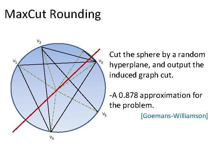
Max. Cut Rounding v 2 v 1 v 3 v 5 v 4 Cut the sphere by a random hyperplane, and output the induced graph cut. -A 0. 878 approximation for the problem. [Goemans-Williamson]

SQUISH AND SOLVE ROUNDING

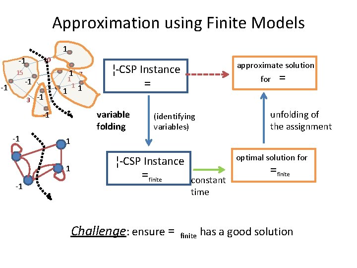
Approximation using Finite Models 1 10 -1 15 -1 -1 3 1 7 1 1 1 -1 1 variable folding -1 -1 for = unfolding of the assignment (identifying variables) 1 1 -1 approximate solution ¦-CSP Instance =finite constant optimal solution for =finite time Challenge: ensure = finite has a good solution

Approximation using Finite Models General Method for CSPs PTAS for dense instances [Frieze-Kannan] For a dense instance =, it is possible to construct finite model =finite OPT(=finite) ≥ (1 -ε) OPT(=) What we will do : SDP value (=finite) > (1 -ε)SDP value (=)

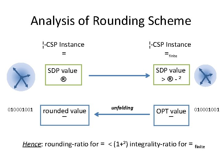
Analysis of Rounding Scheme 01001 ¦-CSP Instance =finite SDP value ® SDP value >®-² rounded value ¯ unfolding OPT value ¯ 01001 Hence: rounding-ratio for = < (1+²) integrality-ratio for = finite

CONSTRUCTING FINITE MODELS (MAXCUT)

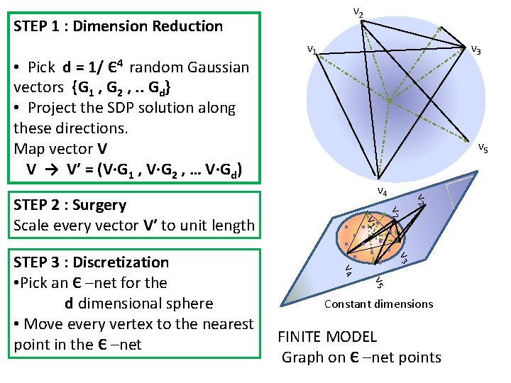
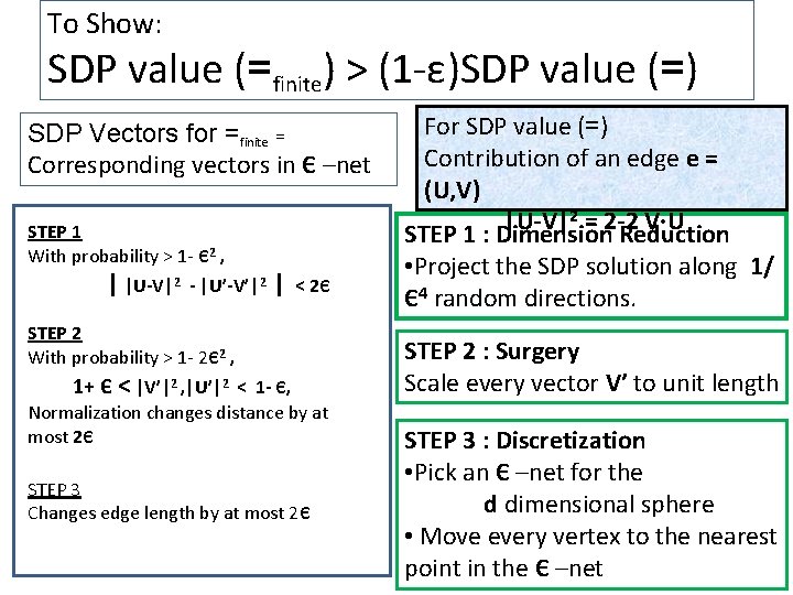
v 2 STEP 1 : Dimension Reduction • Pick d = 1/ Є4 random Gaussian vectors {G 1 , G 2 , . . Gd} • Project the SDP solution along these directions. Map vector V V → V’ = (V∙G 1 , V∙G 2 , … V∙Gd) v 1 v 3 v 5 v 1 v 3 v 4 v 5 STEP 3 : Discretization • Pick an Є –net for the d dimensional sphere • Move every vertex to the nearest point in the Є –net v 2 STEP 2 : Surgery Scale every vector V’ to unit length v 2 v 4 Constant dimensions FINITE MODEL Graph on Є –net points

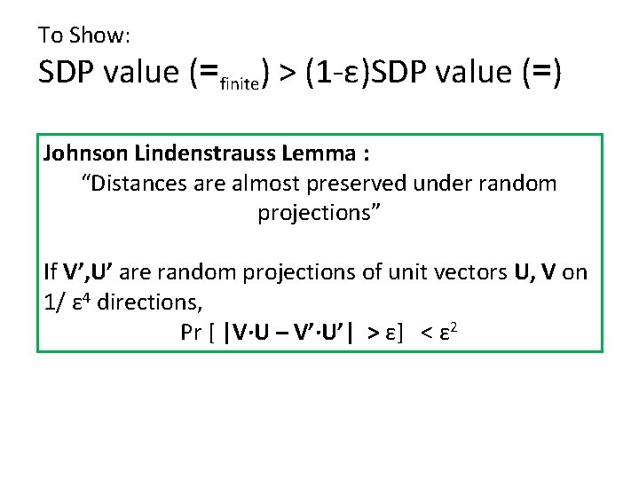
To Show: SDP value (=finite) > (1 -ε)SDP value (=) Johnson Lindenstrauss Lemma : “Distances are almost preserved under random projections” If V’, U’ are random projections of unit vectors U, V on 1/ ε 4 directions, Pr [ |V∙U – V’∙U’| > ε] < ε 2

To Show: SDP value (=finite) > (1 -ε)SDP value (=) SDP Vectors for =finite = Corresponding vectors in Є –net STEP 1 With probability > 1 - Є2 , | |U-V|2 - |U’-V’|2 | < 2Є STEP 2 With probability > 1 - 2Є2 , 1+ Є < |V’|2 , |U’|2 < 1 - Є, Normalization changes distance by at most 2Є STEP 3 Changes edge length by at most 2Є For SDP value (=) Contribution of an edge e = (U, V) 2 = 2 -2 V∙U |U-V| STEP 1 : Dimension Reduction • Project the SDP solution along 1/ Є4 random directions. STEP 2 : Surgery Scale every vector V’ to unit length STEP 3 : Discretization • Pick an Є –net for the d dimensional sphere • Move every vertex to the nearest point in the Є –net

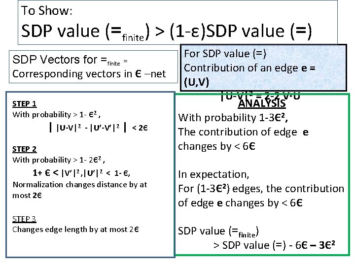
To Show: SDP value (=finite) > (1 -ε)SDP value (=) SDP Vectors for =finite = Corresponding vectors in Є –net STEP 1 With probability > 1 - Є2 , | |U-V|2 - |U’-V’|2 | < 2Є STEP 2 With probability > 1 - 2Є2 , 1+ Є < |V’|2 , |U’|2 < 1 - Є, Normalization changes distance by at most 2Є STEP 3 Changes edge length by at most 2Є For SDP value (=) Contribution of an edge e = (U, V) |U-V|2 = 2 -2 V∙U ANALYSIS With probability 1 -3Є2, The contribution of edge e changes by < 6Є In expectation, For (1 -3Є2) edges, the contribution of edge e changes by < 6Є SDP value (=finite) > SDP value (=) - 6Є – 3Є2

Generic Rounding For CSPs [Raghavendra Steurer 08] For any CSP ¦ and any ²>0, there exists an efficient algorithm A, rounding – ratio. A ( ¦ ) (approximation ratio) (1 -²) integrality gap = ≥ of a natural SDP ( ¦ ) (SDP is optimal under UGC) Drawbacks Unifies a large number of existing rounding schemes, • Running Time(A) and theover resulting algorithm A as On CSP alphabet size q, arity k good as all known algorithms for CSPs (without dependence on n) • No explicit approximation ratio

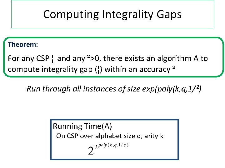
Computing Integrality Gaps Theorem: For any CSP ¦ and any ²>0, there exists an algorithm A to compute integrality gap (¦) within an accuracy ² Run through all instances of size exp(poly(k, q, 1/²) Running Time(A) On CSP over alphabet size q, arity k

Rounding Schemes via Dictatorship Tests [R, 2008]

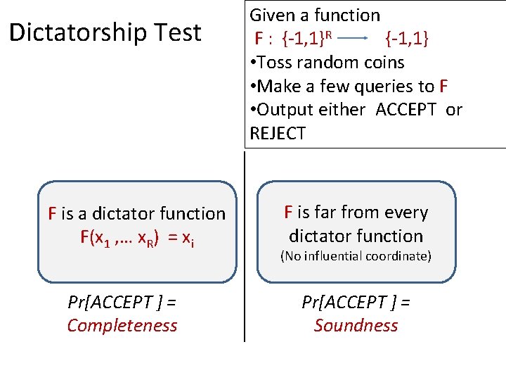
Dictatorship Test F is a dictator function F(x 1 , … x. R) = xi Pr[ACCEPT ] = Completeness Given a function F : {-1, 1}R {-1, 1} • Toss random coins • Make a few queries to F • Output either ACCEPT or REJECT F is far from every dictator function (No influential coordinate) Pr[ACCEPT ] = Soundness

UG Hardness Rule of Thumb: [Khot-Kindler-Mossel-O’Donnell] A dictatorship test where • Completeness = c and Soundness = αc • the verifier’s tests are predicates from a CSP Λ It is UG-hard to approximate CSP Λ to a factor better than α

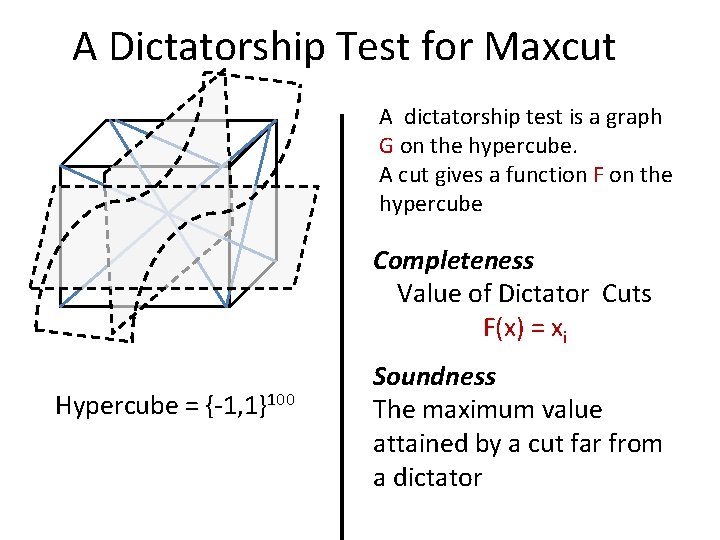
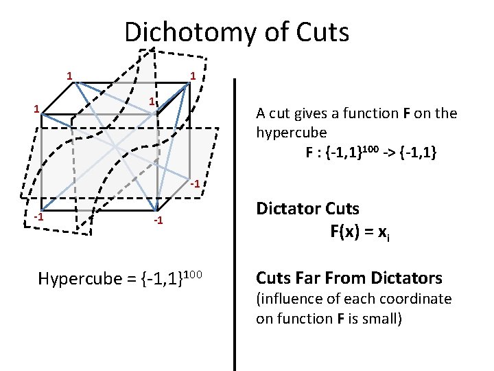
A Dictatorship Test for Maxcut A dictatorship test is a graph G on the hypercube. A cut gives a function F on the hypercube Completeness Value of Dictator Cuts F(x) = xi Hypercube = {-1, 1}100 Soundness The maximum value attained by a cut far from a dictator

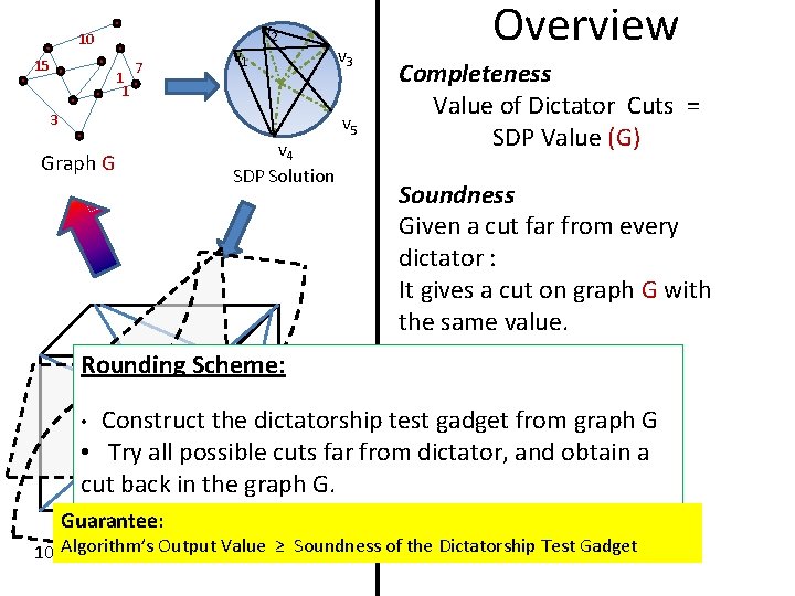
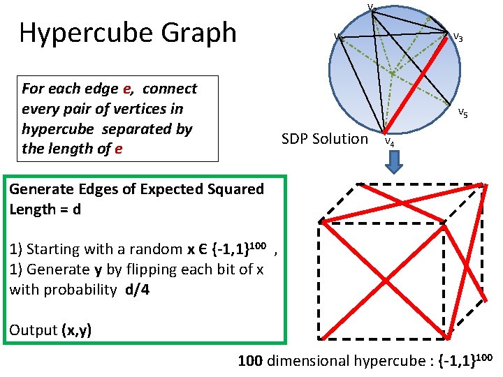
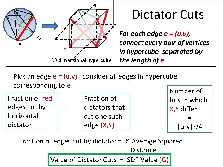
10 15 1 1 7 v 1 v 2 3 Graph G v 4 SDP Solution v 3 v 5 Overview Completeness Value of Dictator Cuts = SDP Value (G) Soundness Given a cut far from every dictator : It gives a cut on graph G with the same value. Rounding Scheme: Construct the dictatorship test gadget from graph G • Try all possible cuts far from dictator, and obtain a cut back in the graph G. • Guarantee: Value ≥ Soundness of the Dictatorship Test Gadget 100 Algorithm’s dimensional. Output hypercube

UG Hardness Dictatorship Test Completeness C Soundness S [KKMO] UG Hardness “On instances, with value C, it is NP-hard to output a solution of value S, assuming UGC” In our case, Completeness = SDP Value (G) Soundness < Algorithm’s Output Cant get better approximation assuming UGC!

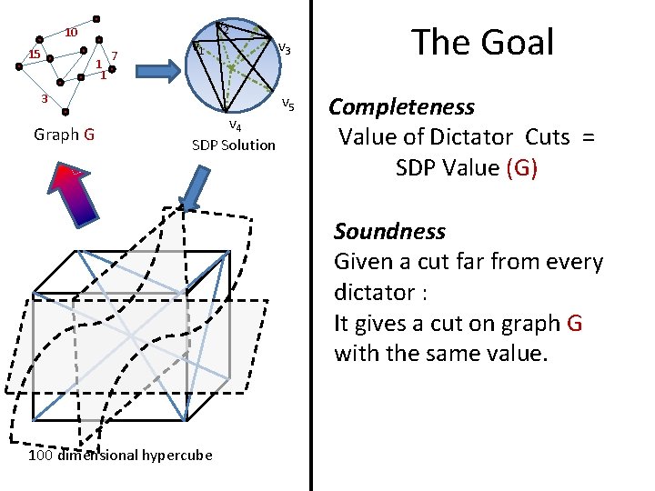
10 15 1 1 7 v 1 v 2 3 Graph G v 4 SDP Solution v 3 v 5 The Goal Completeness Value of Dictator Cuts = SDP Value (G) Soundness Given a cut far from every dictator : It gives a cut on graph G with the same value. 100 dimensional hypercube

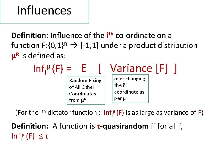
Influences Definition: Influence of the ith co-ordinate on a function F: {0, 1}R [-1, 1] under a product distribution μR is defined as: Infiμ (F) = E [ Variance [F] ] Random Fixing of All Other Coordinates from μR-1 over changing the ith coordinate as per μ (For the ith dictator function : Infiμ (F) is as large as variance of F) Definition: A function is τ-quasirandom if for all i, Infiμ (F) ≤ τ

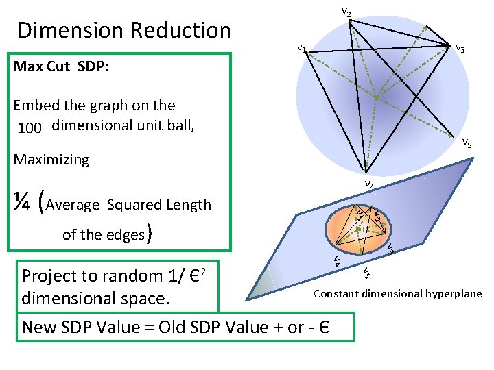
Dimension Reduction v 2 v 1 v 3 Max Cut SDP: Embed the graph on the N - dimensional unit ball, 100 v 5 Maximizing v 4 v 2 v 1 ¼ (Average Squared Length of the edges) v 3 v 4 v 5 Project to random 1/ Є2 Constant dimensional hyperplane dimensional space. New SDP Value = Old SDP Value + or - Є

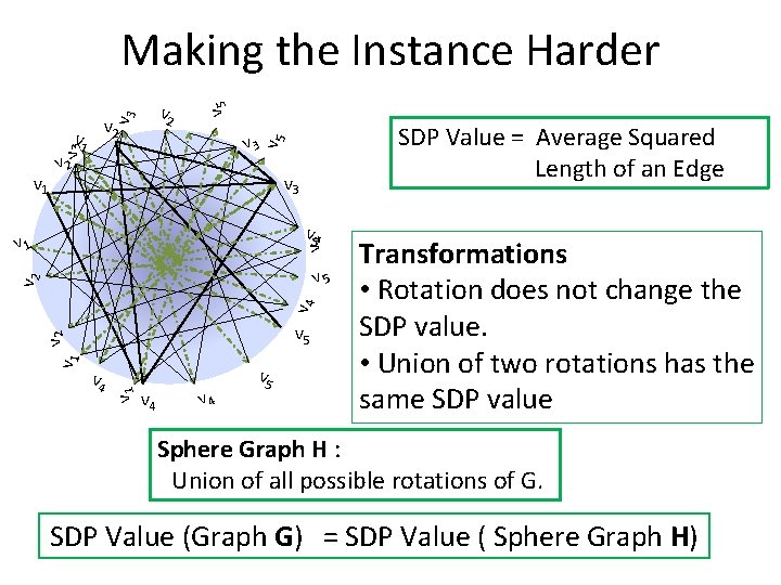
v 3 v 2 v 1 v 2 SDP Value = Average Squared Length of an Edge v 5 v 3 v 1 v 5 Making the Instance Harder v 3 v 4 v 1 v 4 v 2 v 5 v 4 v 1 v 2 v 5 v 4 v 5 Transformations • Rotation does not change the SDP value. • Union of two rotations has the same SDP value Sphere Graph H : Union of all possible rotations of G. SDP Value (Graph G) = SDP Value ( Sphere Graph H)

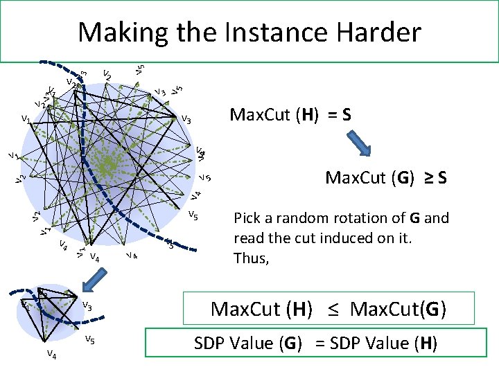
v 3 v 2 v 5 v 3 v 1 v 5 Making the Instance Harder v 1 v 2 Max. Cut (H) = S v 3 v 4 v 1 Max. Cut (G) ≥ S v 4 v 2 v 5 v 1 v 2 v 4 v 1 v 2 v 5 v 4 v 3 v 5 v 4 v 5 Pick a random rotation of G and read the cut induced on it. Thus, Max. Cut (H) ≤ Max. Cut(G) SDP Value (G) = SDP Value (H)

Hypercube Graph For each edge e, connect every pair of vertices in hypercube separated by the length of e v 2 v 1 v 3 v 5 SDP Solution v 4 Generate Edges of Expected Squared Length = d 1) Starting with a random x Є {-1, 1}100 , 1) Generate y by flipping each bit of x with probability d/4 Output (x, y) 100 dimensional hypercube : {-1, 1}100

Dichotomy of Cuts 1 1 A cut gives a function F on the hypercube F : {-1, 1}100 -> {-1, 1} -1 -1 -1 Hypercube = {-1, 1}100 Dictator Cuts F(x) = xi Cuts Far From Dictators (influence of each coordinate on function F is small)

v 1 v 2 X v u v 5 Y 100 dimensional hypercube Dictator Cuts For each edge e = (u, v), connect every pair of vertices in hypercube separated by the length of e Pick an edge e = (u, v), consider all edges in hypercube corresponding to e Number of Fraction of red Fraction of bits in which edges cut by = dictators that = X, Y differ horizontal cut one such = dictator. edge (X, Y) |u-v|2/4 Fraction of edges cut by dictator = ¼ Average Squared Distance Value of Dictator Cuts = SDP Value (G)

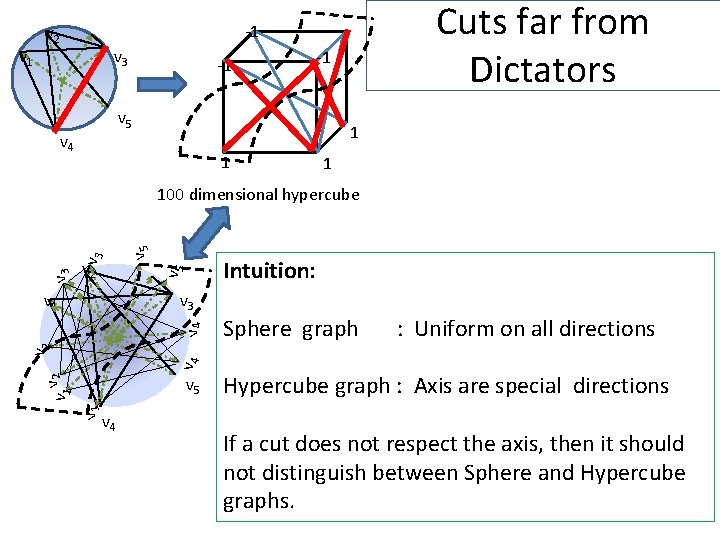
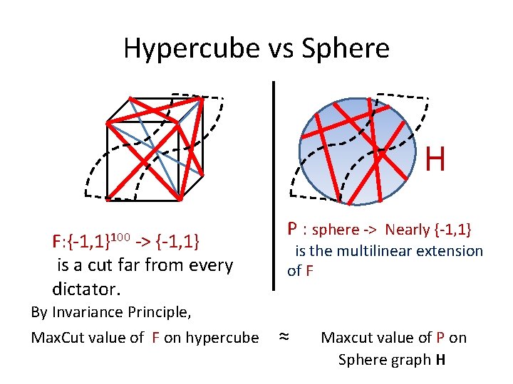
v 1 Cuts far from Dictators -1 v 2 v 3 -1 -1 v 5 v 4 1 1 1 v 5 v 2 v 5 v 3 100 dimensional hypercube v 3 Sphere graph : Uniform on all directions v 1 v 2 v 4 v 1 Intuition: v 1 v 5 v 4 Hypercube graph : Axis are special directions If a cut does not respect the axis, then it should not distinguish between Sphere and Hypercube graphs.

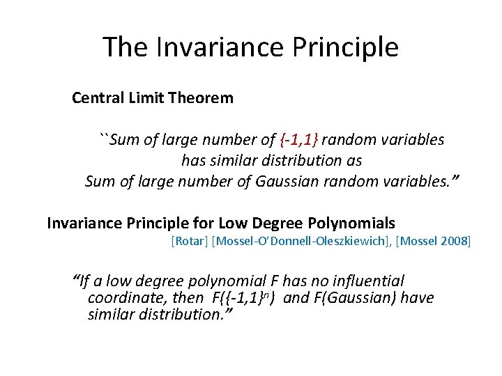
The Invariance Principle Central Limit Theorem ``Sum of large number of {-1, 1} random variables has similar distribution as Sum of large number of Gaussian random variables. ” Invariance Principle for Low Degree Polynomials [Rotar] [Mossel-O’Donnell-Oleszkiewich], [Mossel 2008] “If a low degree polynomial F has no influential coordinate, then F({-1, 1}n) and F(Gaussian) have similar distribution. ”

Hypercube vs Sphere H F: {-1, 1}100 -> {-1, 1} is a cut far from every dictator. By Invariance Principle, Max. Cut value of F on hypercube P : sphere -> Nearly {-1, 1} is the multilinear extension of F ≈ Maxcut value of P on Sphere graph H

Rounding SDP Hierarchies via Correlation [Barak, R, Steurer 2011] [R, Tan 2011]

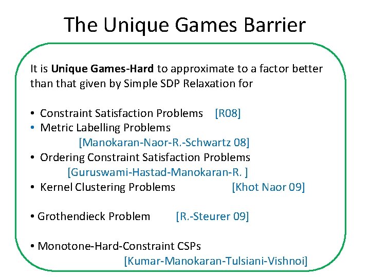
The Unique Games Barrier It is Unique Games-Hard to approximate to a factor better than that given by Simple SDP Relaxation for • Constraint Satisfaction Problems [R 08] • Metric Labelling Problems [Manokaran-Naor-R. -Schwartz 08] • Ordering Constraint Satisfaction Problems [Guruswami-Hastad-Manokaran-R. ] • Kernel Clustering Problems [Khot Naor 09] • Grothendieck Problem [R. -Steurer 09] • Monotone-Hard-Constraint CSPs [Kumar-Manokaran-Tulsiani-Vishnoi]

For the non-believers [R-Steurer 09] Unconditionally, Adding all valid constraints on at most 2^O((loglogn)1/4) variables to the simple SDP does not improve the approximation ratio for Constraint Satisfaction Problems Ordering Constraint Satisfaction Problems Metric Labelling Problems Kernel Clustering Problems Grothendieck Problem

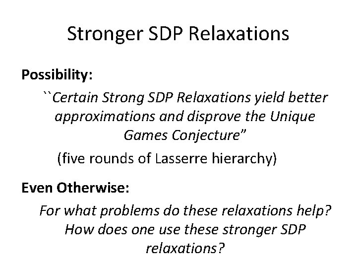
Stronger SDP Relaxations Possibility: ``Certain Strong SDP Relaxations yield better approximations and disprove the Unique Games Conjecture” (five rounds of Lasserre hierarchy) Even Otherwise: For what problems do these relaxations help? How does one use these stronger SDP relaxations?

Difficulty Successes of Stronger SDP Relaxations: • [Arora-Rao-Vazirani] used an SDP with triangle inequalities to improve approximation for Sparsest Cut from log n to sqrt(log n). • Stronger SDPs for better approximations for graph and hypergraph independent set in [Chlamtac] [Arora-Charikar-Chlamtac] [Chlamtac-Singh] Very few general techniques to extract the power of stronger SDP relaxations. .

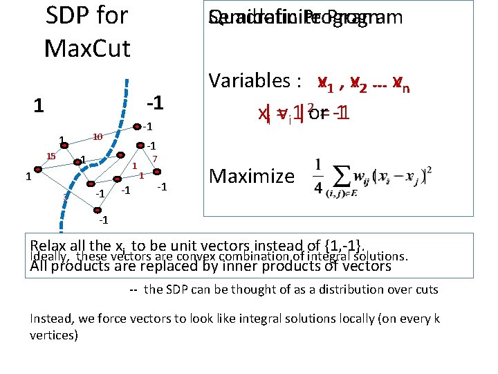
SDP for Max. Cut Semidefinite Quadratic Program -1 1 10 1 15 -1 -1 1 3 -1 Variables : xv 1 , xv 2 … xvn x|i =vi 1|2 or= -1 1 -1 7 1 -1 Maximize -1 Relax all the xi to be unit vectors instead of {1, -1}. Ideally, these vectors are convex combination of integral solutions. All products are replaced by inner products of vectors -- the SDP can be thought of as a distribution over cuts Instead, we force vectors to look like integral solutions locally (on every k vertices)

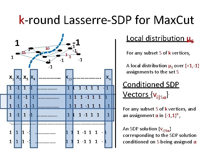
k-round Lasserre-SDP for Max. Cut 1 1 15 1 3 1 -1 10 -1 -17 1 Local distribution μS For any subset S of k vertices, -1 X 2 X 3 X 4 ……………. . X 15 …………………. Xn 1 -1 ……………. . 1 1 1 -1 -1 -1 ……………. . 1 1 1 -1 1 1 -1 ……………. . 1 1 1 - 1 -………………………………… 1 1 1 -1 ……………. . 1 1 1 -1 1 1 - 1 A local distribution μS over {+1, -1} assignments to the set S Conditioned SDP Vectors {vi|Sα} For any subset S of k vertices, and an assignment α in {-1, 1}k , An SDP solution {vi|Sα} corresponding to the SDP solution conditioned on S being assigned α

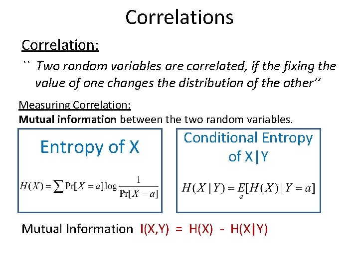
Correlations Correlation: `` Two random variables are correlated, if the fixing the value of one changes the distribution of the other’’ Measuring Correlation: Mutual information between the two random variables. Entropy of X Conditional Entropy of X|Y Mutual Information I(X, Y) = H(X) - H(X|Y)

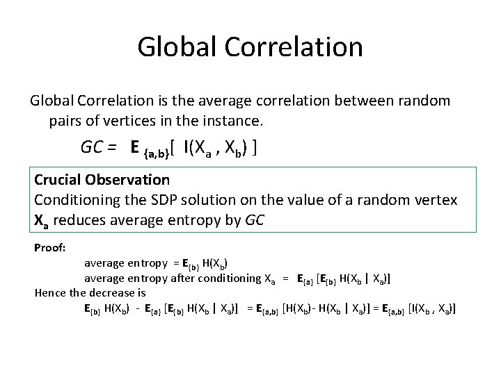
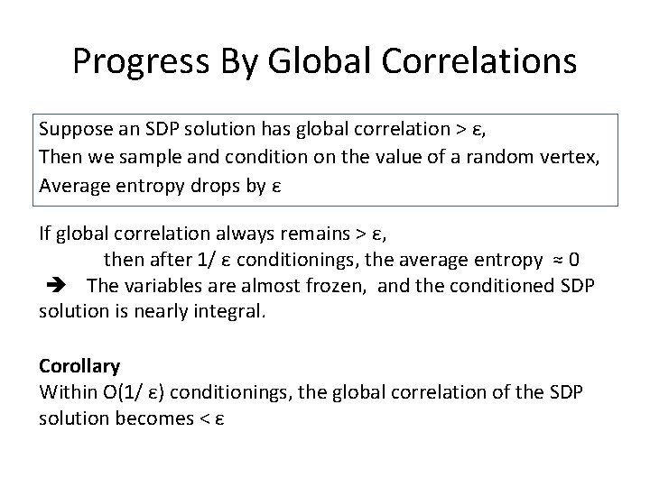
Global Correlation is the average correlation between random pairs of vertices in the instance. GC = E {a, b}[ I(Xa , Xb) ] Crucial Observation Conditioning the SDP solution on the value of a random vertex Xa reduces average entropy by GC Proof: average entropy = E{b} H(Xb) average entropy after conditioning Xa = E{a} [E{b} H(Xb | Xa)] Hence the decrease is E{b} H(Xb) - E{a} [E{b} H(Xb | Xa)] = E{a, b} [H(Xb)- H(Xb | Xa)] = E{a, b} [I(Xb , Xa)]

Progress By Global Correlations Suppose an SDP solution has global correlation > ε, Then we sample and condition on the value of a random vertex, Average entropy drops by ε If global correlation always remains > ε, then after 1/ ε conditionings, the average entropy ≈ 0 The variables are almost frozen, and the conditioned SDP solution is nearly integral. Corollary Within O(1/ ε) conditionings, the global correlation of the SDP solution becomes < ε

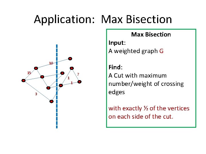
Application: Max Bisection Input: A weighted graph G 10 15 7 1 1 3 Find: A Cut with maximum number/weight of crossing edges with exactly ½ of the vertices on each side of the cut.

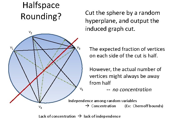
Halfspace Rounding? Cut the sphere by a random hyperplane, and output the induced graph cut. v 2 v 1 v 3 v 5 v 4 The expected fraction of vertices on each side of the cut is half. However, the actual number of vertices might always be away from half -- no concentration Independence among random variables Concentration (Ex: Chernoff bounds) Lack of concentration lack of independence

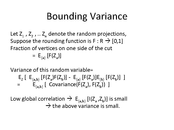
Bounding Variance Let Z 1 , Z 2 , . . Zn denote the random projections, Suppose the rounding function is F : R [0, 1] Fraction of vertices on one side of the cut = E{a} [F(Za)] Variance of this random variable= EZ [ E{a, b} [F(Za)F(Zb)] - E{a} [F(Za)]E{b} [F(Zb)] ] = E{a, b} [ Covariance(F(Za), F(Zb)) ] Low global correlation E{a, b} [I(Za , Zb)] is small the above variance is small.

CSPs with Global Cardinality Constraint [R, Tan 2011] Given an instance of Max Bisection/Min Bisection with value 1 -ε, there is an algorithm running in time npoly(1/ε) that finds a solution of value 1 -O(ε 1/2) [R, Tan 2011] For every CSP with global cardinality constraint, there is a corresponding dictatorship test whose Soundness/Completeness = Integrality gap of poly(1/ ε) - round Lasserre SDP.

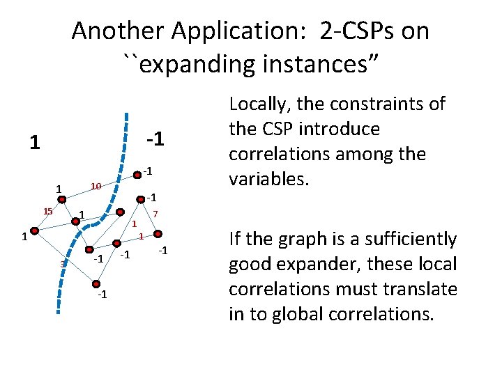
Another Application: 2 -CSPs on ``expanding instances” -1 10 1 15 -1 1 7 1 1 1 3 -1 -1 -1 Locally, the constraints of the CSP introduce correlations among the variables. -1 If the graph is a sufficiently good expander, these local correlations must translate in to global correlations.

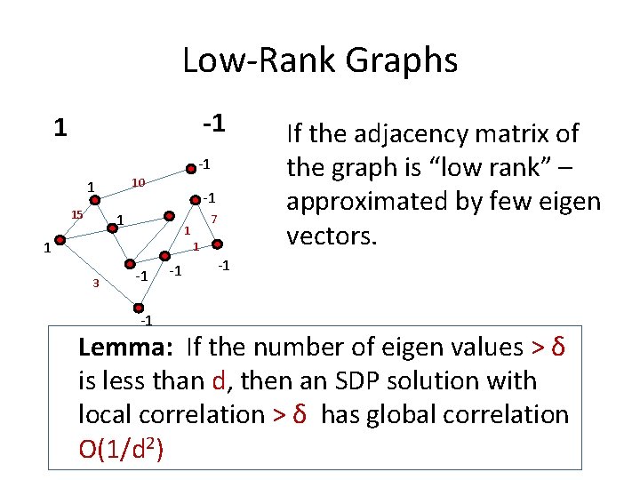
Low-Rank Graphs -1 10 1 15 -1 1 7 1 1 1 3 -1 -1 -1 If the adjacency matrix of the graph is “low rank” – approximated by few eigen vectors. -1 Lemma: If the number of eigen values > δ is less than d, then an SDP solution with local correlation > δ has global correlation O(1/d 2)

2 -CSP on random constraint graphs [Barak-Raghavendra-Steurer] Given an instance of 2 -CSP whose constraint graph is a degree d random graph, poly(1/ε, k, d) round Lasserre SDP hierarchy has value < Optimum + od(1)

Another Application Subexponential Time Algorithm for Unique Games [Arora-Barak-Steurer] Given an instance of Unique Games with value 1 -ε, in time exp(nε), the algorithm finds a solution of value 1 -εc Used a combination of brute force and spectral decomposition, but no SDPs Subexponential Time Algorithm for Unique Games via SDPs [Barak-Raghavendra-Steurer] [Guruswami-Sinop] Given an instance of Unique Games such that n. O(ε) – rounds of SDP hierarchy has value with value 1 -ε, there exists an assignment of value 1 -εc

Future Work Can one use local-global correlations to prove [Arora-Rao-Vazirani] or something weaker? subexponential time algorithms beating the current best for Max. Cut, Sparsest Cut?

Thank You

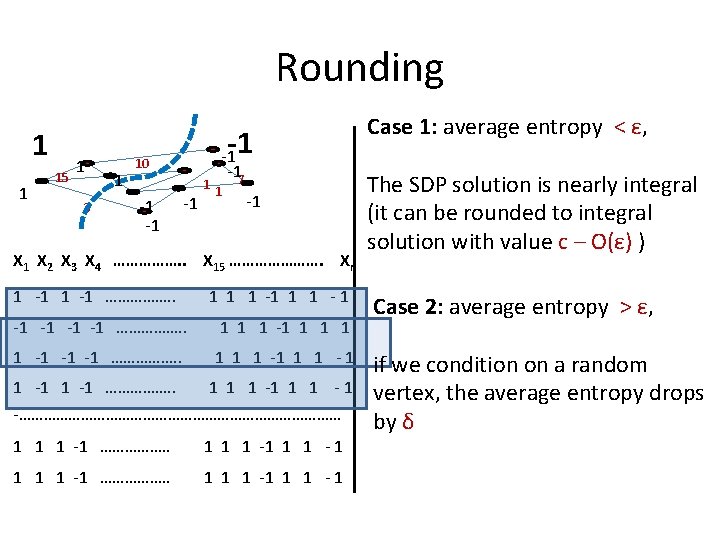
Rounding 1 1 15 1 3 1 -1 10 -1 -17 1 -1 X 2 X 3 X 4 ……………. . X 15 …………………. Xn 1 -1 ……………. . 1 1 1 - 1 -1 -1 ……………. . 1 1 1 -1 -1 -1 ……………. . 1 1 1 -1 ……………. . 1 1 1 - 1 -………………………………… 1 1 1 -1 ……………. . 1 1 1 -1 1 1 - 1 Case 1: average entropy < ε, The SDP solution is nearly integral (it can be rounded to integral solution with value c – O(ε) ) Case 2: average entropy > ε, if we condition on a random vertex, the average entropy drops by δ

Main Theorem (Informal): If an instance I of a problem satisfies (c, ε, δ)global correlation property, Then, (1/δ)-round SDP solution on the instance I is within O(ε) of the integral value. Do instances have this global correlation property arise?