Generalized Linear Mixed Models to analyse data from

Generalized Linear Mixed Models to analyse data from Respondent. Driven Sampling Märt Möls, Krista Fischer, Anneli Uusküla, Helle Kilgi Tartu University, Estonia

Hard-to-reach populations n n n Intravenous Drug Users Example: Estonian Intravenous Drug Users Survey (Data collection 2005) Commercial Sex Workers Example: Estonian Commercial Sex Workers Survey (Data collection 2006) gay men; street youth; homeless; bayesian etc.

Respondent-Driven Sampling (RDS)

Respondent-Driven Sampling (RDS)

Respondent-Driven Sampling (RDS)

Respondent-Driven Sampling (RDS)

Respondent-Driven Sampling (RDS)

Respondent-Driven Sampling (RDS)

Respondent-Driven Sampling (RDS)

Respondent-Driven Sampling (RDS)

Estonian IDU Study

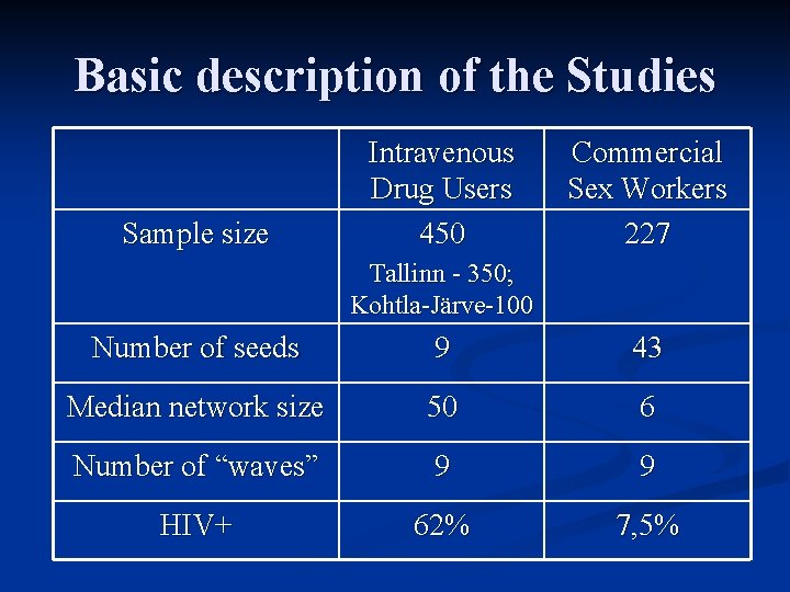
Basic description of the Studies Sample size Intravenous Drug Users 450 Commercial Sex Workers 227 Tallinn - 350; Kohtla-Järve-100 Number of seeds 9 43 Median network size 50 6 Number of “waves” 9 9 HIV+ 62% 7, 5%

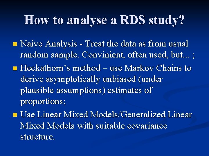
How to analyse a RDS study? Naive Analysis - Treat the data as from usual random sample. Convinient, often used, but. . . ; n Heckathorn’s method – use Markov Chains to derive asymptotically unbiased (under plausible assumptions) estimates of proportions; n Use Linear Mixed Models/Generalized Linear Mixed Models with suitable covariance structure. n

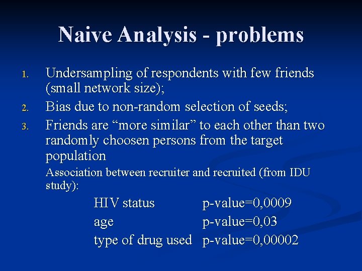
Naive Analysis - problems 1. 2. 3. Undersampling of respondents with few friends (small network size); Bias due to non-random selection of seeds; Friends are “more similar” to each other than two randomly choosen persons from the target population Association between recruiter and recruited (from IDU study): HIV status age type of drug used p-value=0, 0009 p-value=0, 03 p-value=0, 00002

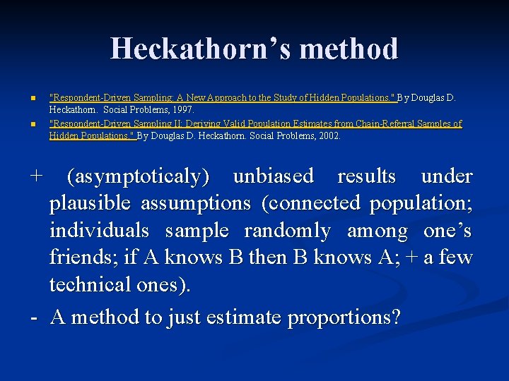
Heckathorn’s method n n "Respondent-Driven Sampling: A New Approach to the Study of Hidden Populations. " By Douglas D. Heckathorn. Social Problems, 1997. "Respondent-Driven Sampling II: Deriving Valid Population Estimates from Chain-Referral Samples of Hidden Populations. " By Douglas D. Heckathorn. Social Problems, 2002. + (asymptoticaly) unbiased results under plausible assumptions (connected population; individuals sample randomly among one’s friends; if A knows B then B knows A; + a few technical ones). - A method to just estimate proportions?

Linear Mixed Models / GLMM AIM: To provide classical modelling possibilities to analyse samples collected based on a RDS design.

Remedy 1 - Undersampling 1. Undersampling can be corrected using weighted averages or related techniques (estimation of certain linear functions of parameters). Corrections are regularly applied if stratified random sampling has been used, for example.

Distribution of network sizes

Correction for undersampling 1. Include network size to the model of interest, eg. : logit(P(HIV+|NS)) = c+f(NS) 2. Integrate NS out from the final result based on the estimated proportions of network sizes, eg: P(HIV+) = ∑ P(HIV+|NS=i) P(NS=i) 3. Use delta method to calculate se for logistic regression; exact calculations for linear models.

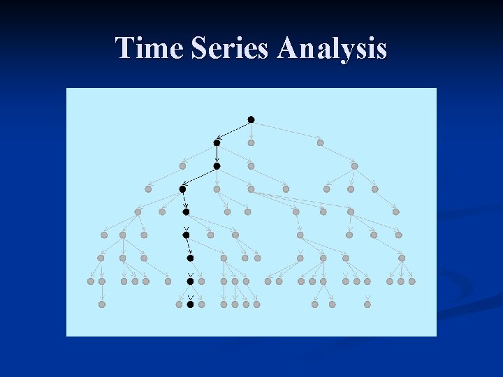
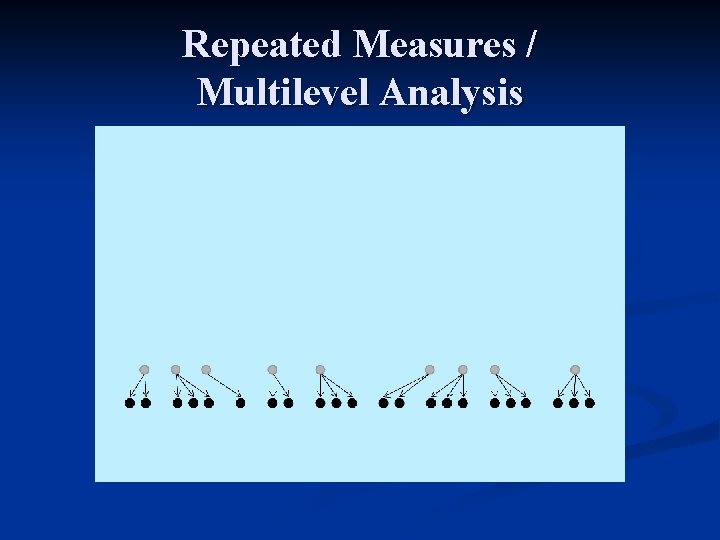
There is nothing new in analysing correlated observations. For example, one can use

Time Series Analysis

Repeated Measures / Multilevel Analysis

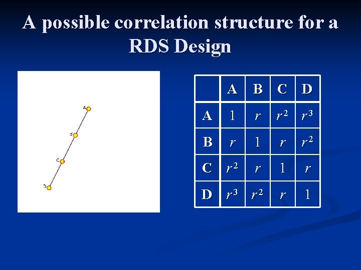
A possible correlation structure for a RDS Design A B C D A 1 r r 2 r 3 B r 1 r r 2 C r 2 r 1 r D r 3 r 2 r 1

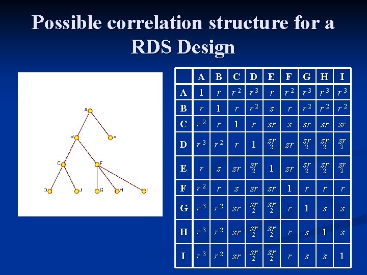
Possible correlation structure for a RDS Design A B C D E F A 1 r r 2 r 3 r 3 B r 1 r r 2 s r r 2 r 2 C r 2 r 1 r sr sr sr D r 3 r 2 r 1 sr sr sr 2 2 E r s sr sr 2 F r 2 r s 1 G H I sr sr 2 2 2 sr sr 1 r r r sr G r 3 r 2 sr sr 2 2 r 1 s s sr H r 3 r 2 sr sr 2 2 r s 1 s sr r 3 r 2 sr sr 2 2 r s s 1 I

Some possible modeling approaches using such correlation structure: n Linear Mixed Models n Generalized Latent Variable Models / Generalized Structural Equation Models n. .

Correction for seed selection bias? n n May-be one can consider the seed selection bias as a random “effect” added to the seeds (seeds are correlated to each other due to the random “selection bias” effect); This added random “effect” is propagating (in a decreasing way) along the recruitment path – so the “offsprings” of different seeds start to be less correlated after each new recruitment wave. - Suggested approach is really computer intensive. Estimating linear/generalized linear models by using this kind of correlation structure can really be too slow.

Does it work? Comparison with other methods n Simulations n Does the proposed model fit to the real data? n

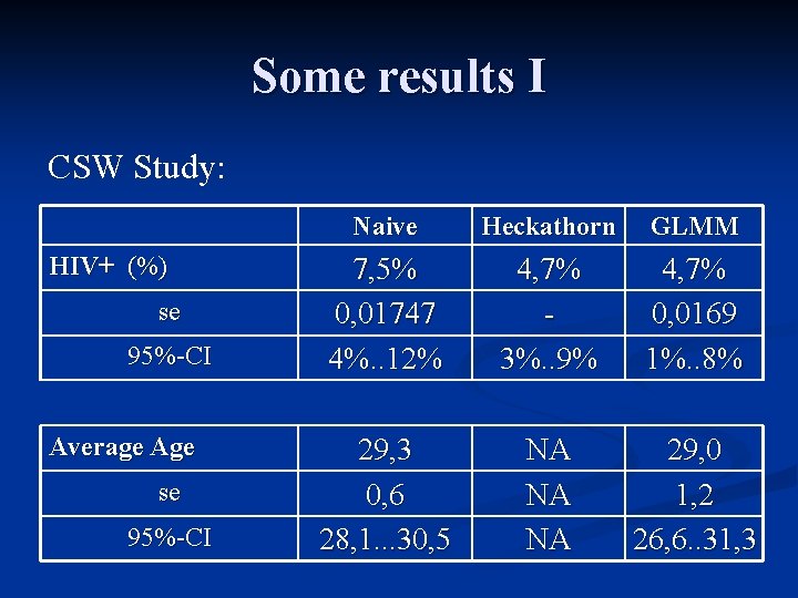
Some results I CSW Study: HIV+ (%) se 95%-CI Average Age se 95%-CI Naive Heckathorn GLMM 7, 5% 0, 01747 4%. . 12% 4, 7% 3%. . 9% 4, 7% 0, 0169 1%. . 8% 29, 3 0, 6 28, 1. . . 30, 5 NA NA NA 29, 0 1, 2 26, 6. . 31, 3

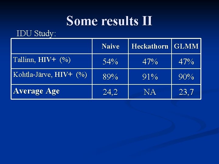
Some results II IDU Study: Naive Heckathorn GLMM Tallinn, HIV+ (%) 54% 47% Kohtla-Järve, HIV+ (%) 89% 91% 90% Average Age 24, 2 NA 23, 7

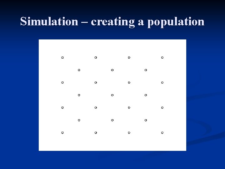
Simulation – creating a population

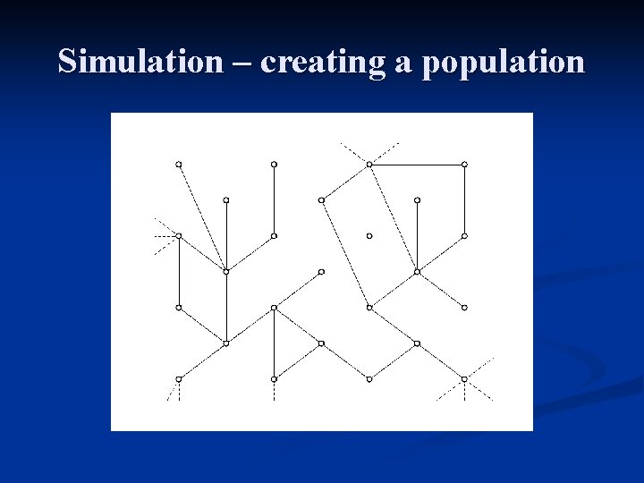
Simulation – creating a population

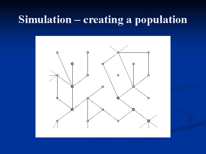
Simulation – creating a population

Simulation – creating a population

Simulation – creating a population

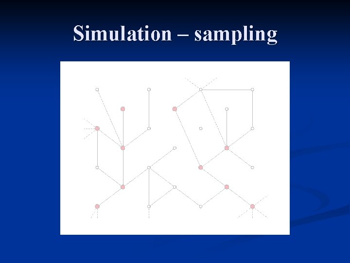
Simulation – sampling

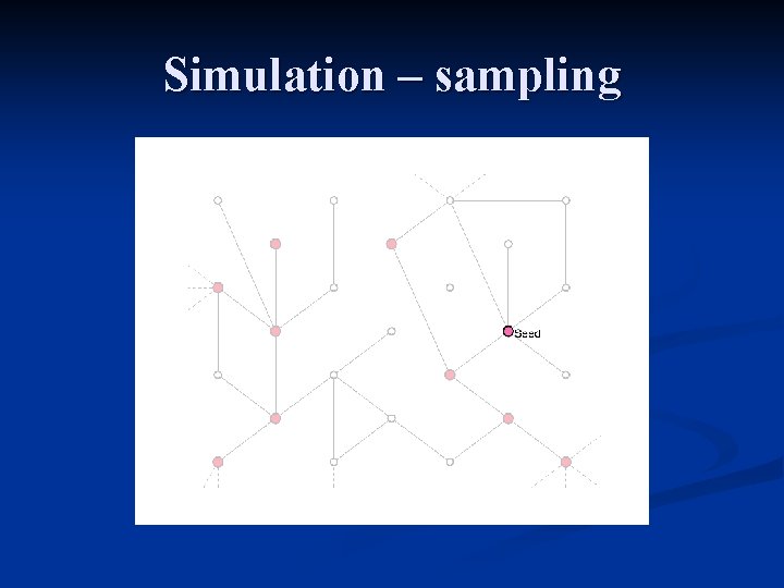
Simulation – sampling

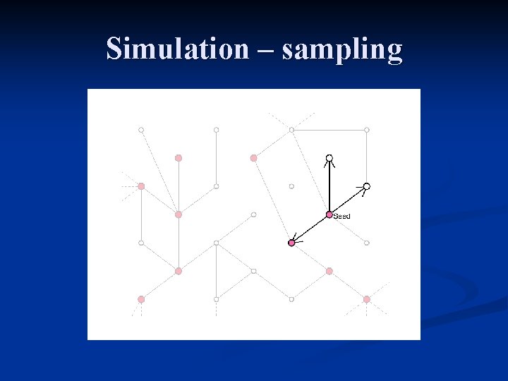
Simulation – sampling

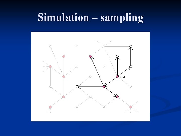
Simulation – sampling

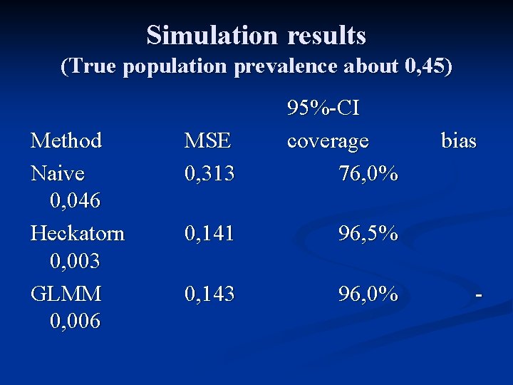
Simulation results (True population prevalence about 0, 45) Method Naive 0, 046 Heckatorn 0, 003 GLMM 0, 006 MSE 0, 313 95%-CI coverage 76, 0% bias 0, 141 96, 5% 0, 143 96, 0% -

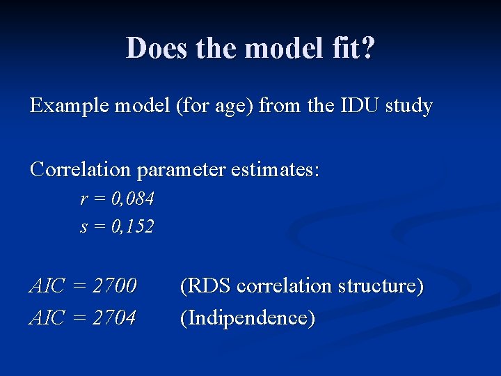
Does the model fit? Example model (for age) from the IDU study Correlation parameter estimates: r = 0, 084 s = 0, 152 AIC = 2700 AIC = 2704 (RDS correlation structure) (Indipendence)

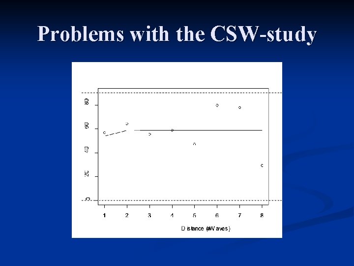
Problems with the CSW-study

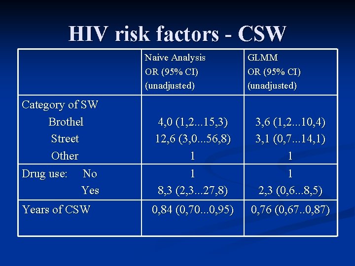
HIV risk factors - CSW Naive Analysis OR (95% CI) (unadjusted) GLMM OR (95% CI) (unadjusted) Category of SW Brothel Street Other Drug use: No Yes 4, 0 (1, 2. . . 15, 3) 12, 6 (3, 0. . . 56, 8) 1 1 8, 3 (2, 3. . . 27, 8) 3, 6 (1, 2. . . 10, 4) 3, 1 (0, 7. . . 14, 1) 1 1 2, 3 (0, 6. . . 8, 5) Years of CSW 0, 84 (0, 70. . . 0, 95) 0, 76 (0, 67. . 0, 87)

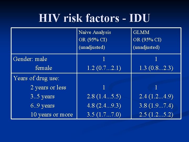
HIV risk factors - IDU Naive Analysis OR (95% CI) (unadjusted) GLMM OR (95% CI) (unadjusted) Gender: male female 1 1. 2 (0. 7. . . 2. 1) 1 1. 3 (0. 8. . . 2. 3) Years of drug use: 2 years or less 3. . 5 years 6. . 9 years 10 years or more 1 2. 8 (1. 4. . . 5. 5) 4. 8 (2. 4. . . 9. 3) 3. 5 (1. 7. 0) 1 2. 4 (1. 2. . . 4. 9) 3. 8 (1. 9. . . 7. 4) 2. 5 (1. 2. . . 5. 2)

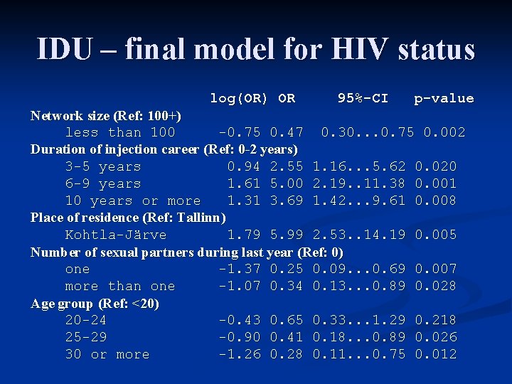
IDU – final model for HIV status log(OR) OR 95%-CI p-value Network size (Ref: 100+) less than 100 -0. 75 0. 47 0. 30. . . 0. 75 0. 002 Duration of injection career (Ref: 0 -2 years) 3 -5 years 0. 94 2. 55 1. 16. . . 5. 62 0. 020 6 -9 years 1. 61 5. 00 2. 19. . 11. 38 0. 001 10 years or more 1. 31 3. 69 1. 42. . . 9. 61 0. 008 Place of residence (Ref: Tallinn) Kohtla-Järve 1. 79 5. 99 2. 53. . 14. 19 0. 005 Number of sexual partners during last year (Ref: 0) one -1. 37 0. 25 0. 09. . . 0. 69 0. 007 more than one -1. 07 0. 34 0. 13. . . 0. 89 0. 028 Age group (Ref: <20) 20 -24 -0. 43 0. 65 0. 33. . . 1. 29 0. 218 25 -29 -0. 90 0. 41 0. 18. . . 0. 89 0. 026 30 or more -1. 26 0. 28 0. 11. . . 0. 75 0. 012

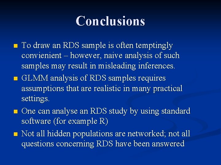
Conclusions n n To draw an RDS sample is often temptingly convienient – however, naive analysis of such samples may result in misleading inferences. GLMM analysis of RDS samples requires assumptions that are realistic in many practical settings. One can analyse an RDS study by using standard software (for example R) Not all hidden populations are networked; not all questions concerning RDS have been answered