GADTs in Haskell ADT vs GADT Algebraic Datatype

GADTs in Haskell

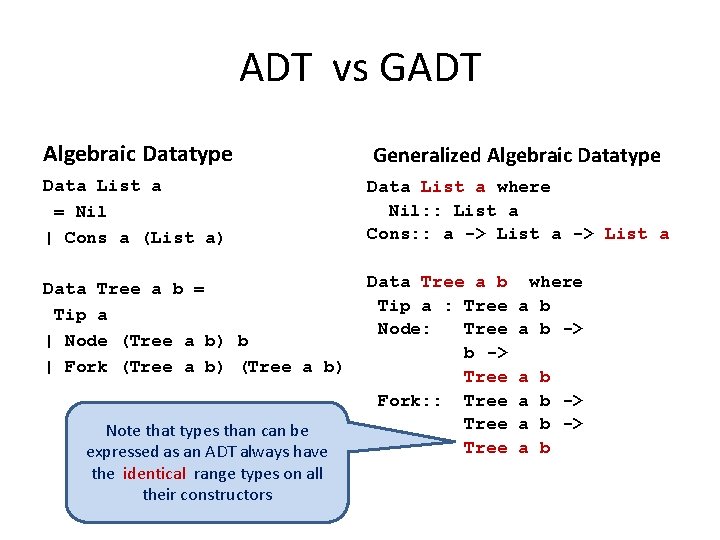
ADT vs GADT Algebraic Datatype Generalized Algebraic Datatype Data List a = Nil | Cons a (List a) Data List a where Nil: : List a Cons: : a -> List a Data Tree a b = Tip a | Node (Tree a b) b | Fork (Tree a b) Data Tree a b Tip a : Tree Node: Tree b -> Tree Fork: : Tree Note that types than can be expressed as an ADT always have the identical range types on all their constructors where a b -> a a b b -> b

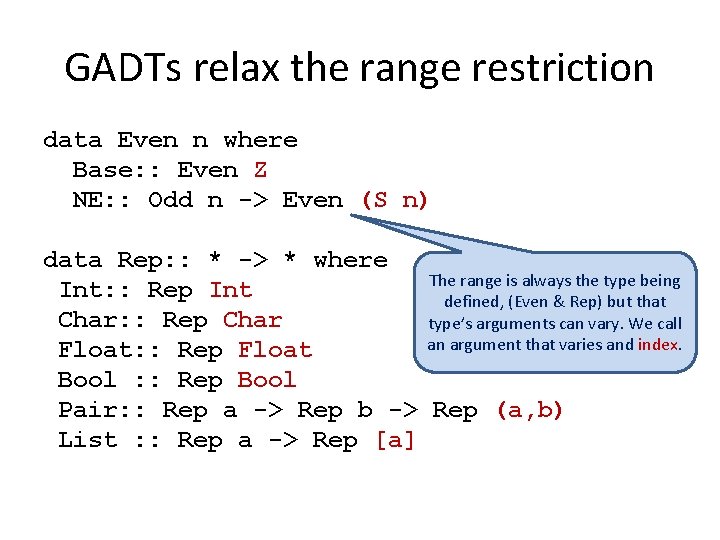
GADTs relax the range restriction data Even n where Base: : Even Z NE: : Odd n -> Even (S n) data Rep: : * -> * where The range is always the type being Int: : Rep Int defined, (Even & Rep) but that Char: : Rep Char type’s arguments can vary. We call an argument that varies and index. Float: : Rep Float Bool : : Rep Bool Pair: : Rep a -> Rep b -> Rep (a, b) List : : Rep a -> Rep [a]

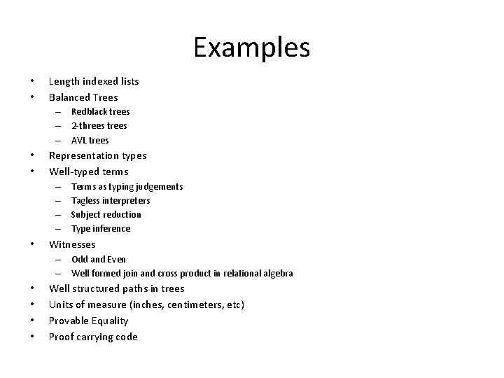
Examples • • Length indexed lists Balanced Trees – Redblack trees – 2 -threes trees – AVL trees • • Representation types Well-typed terms – – • Terms as typing judgements Tagless interpreters Subject reduction Type inference Witnesses – Odd and Even – Well formed join and cross product in relational algebra • • Well structured paths in trees Units of measure (inches, centimeters, etc) Provable Equality Proof carrying code

Length indexed lists data Z data S n Note we introduce uninhabited types that have the structure of the Natural numbers to serve as indexes to LList data LList : : * -> * where LNil: : LList a Z LCons: : a -> LList a n -> LList a (S n) Note the range type is always LList But they differ in the indexes.

Promotion • As of GHC version 7 GHC allows indexes to be ordinary datatypes. • One says the datatype is promoted to the type level. • This is very usefull, as it enforces a typing system on the indexes. – For example does (LList Int String) make any sense. The index is supposed to be drawn from Z and S

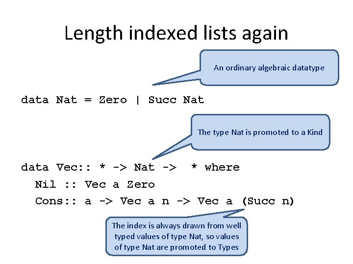
Length indexed lists again An ordinary algebraic datatype data Nat = Zero | Succ Nat The type Nat is promoted to a Kind data Vec: : * -> Nat -> * where Nil : : Vec a Zero Cons: : a -> Vec a n -> Vec a (Succ n) The index is always drawn from well typed values of type Nat, so values of type Nat are promoted to Types

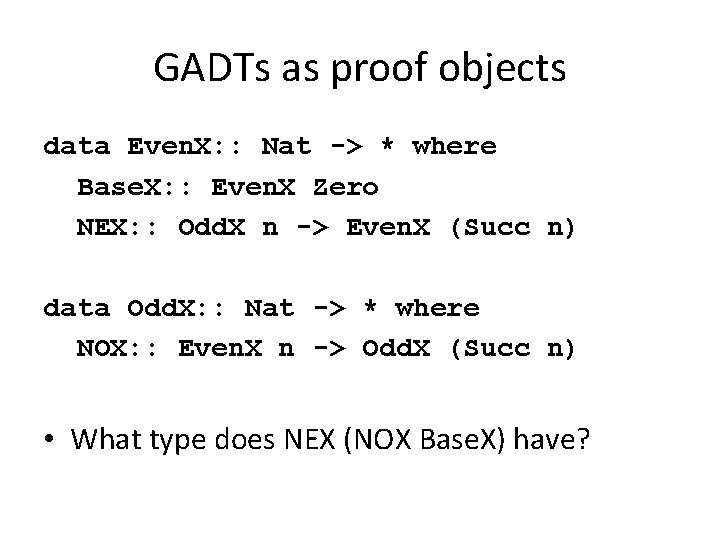
GADTs as proof objects data Even. X: : Nat -> * where Base. X: : Even. X Zero NEX: : Odd. X n -> Even. X (Succ n) data Odd. X: : Nat -> * where NOX: : Even. X n -> Odd. X (Succ n) • What type does NEX (NOX Base. X) have?

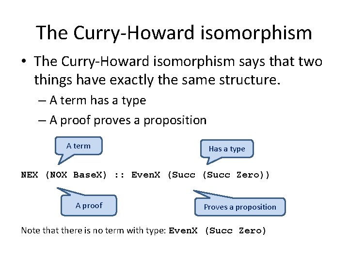
The Curry-Howard isomorphism • The Curry-Howard isomorphism says that two things have exactly the same structure. – A term has a type – A proof proves a proposition A term Has a type NEX (NOX Base. X) : : Even. X (Succ Zero)) A proof Proves a proposition Note that there is no term with type: Even. X (Succ Zero)

Proofs and witnesses • GADTs make the Curry-Howard isomorphism useful in Haskell. • Sometime we say a term “witnesses” a property. I. e the term NEX (NOX Base. X) witnesses that 2 is even. • We use GADTs has indexes to show that some things are not possible.

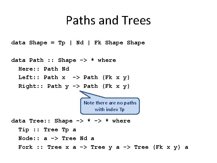
Paths and Trees data Shape = Tp | Nd | Fk Shape data Path : : Shape -> * where Here: : Path Nd Left: : Path x -> Path (Fk x y) Right: : Path y -> Path (Fk x y) Note there are no paths with index Tp data Tree: : Shape -> * where Tip : : Tree Tp a Node: : a -> Tree Nd a Fork : : Tree x a -> Tree y a -> Tree (Fk x y) a

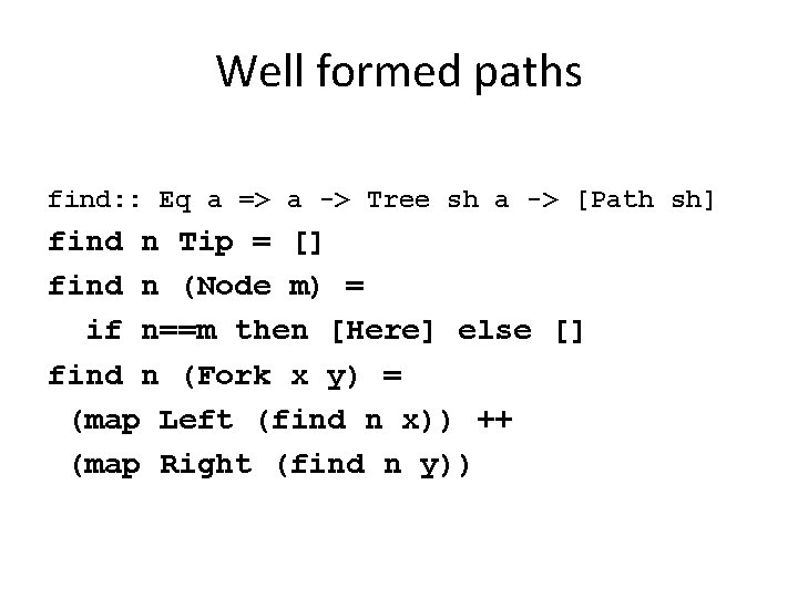
Well formed paths find: : Eq a => a -> Tree sh a -> [Path sh] find n Tip = [] find n (Node m) = if n==m then [Here] else [] find n (Fork x y) = (map Left (find n x)) ++ (map Right (find n y))

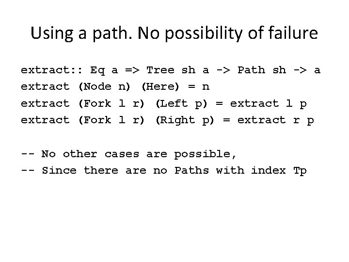
Using a path. No possibility of failure extract: : Eq a => Tree sh a -> Path sh -> a extract (Node n) (Here) = n extract (Fork l r) (Left p) = extract l p extract (Fork l r) (Right p) = extract r p -- No other cases are possible, -- Since there are no Paths with index Tp

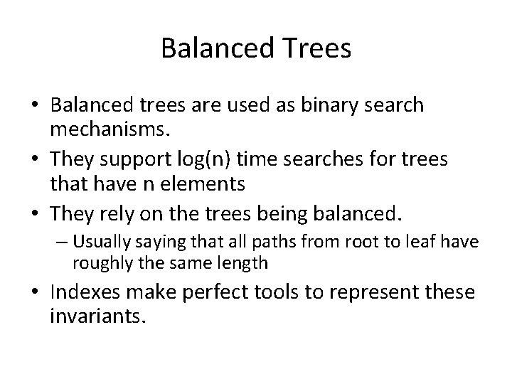
Balanced Trees • Balanced trees are used as binary search mechanisms. • They support log(n) time searches for trees that have n elements • They rely on the trees being balanced. – Usually saying that all paths from root to leaf have roughly the same length • Indexes make perfect tools to represent these invariants.

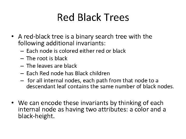
Red Black Trees • A red-black tree is a binary search tree with the following additional invariants: – – – Each node is colored either red or black The root is black The leaves are black Each Red node has Black children for all internal nodes, each path from that node to a descendant leaf contains the same number of black nodes. • We can encode these invariants by thinking of each internal node as having two attributes: a color and a black-height.

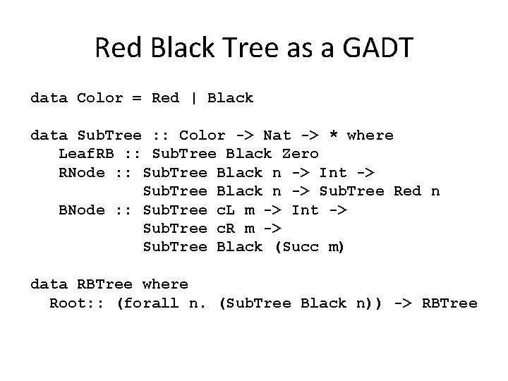
Red Black Tree as a GADT data Color = Red | Black data Sub. Tree : : Color -> Nat -> * where Leaf. RB : : Sub. Tree Black Zero RNode : : Sub. Tree Black n -> Int -> Sub. Tree Black n -> Sub. Tree Red n BNode : : Sub. Tree c. L m -> Int -> Sub. Tree c. R m -> Sub. Tree Black (Succ m) data RBTree where Root: : (forall n. (Sub. Tree Black n)) -> RBTree

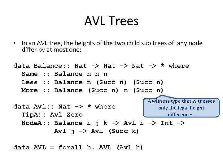
AVL Trees • In an AVL tree, the heights of the two child sub trees of any node differ by at most one; data Balance: : Nat -> * where Same : : Balance n n n Less : : Balance n (Succ n) More : : Balance (Succ n) n (Succ n) A witness type that witnesses only the legal height differences. data Avl: : Nat -> * where Tip. A: : Avl Zero Node. A: : Balance i j k -> Avl i -> Int -> Avl j -> Avl (Succ k) data AVL = forall h. AVL (Avl h)

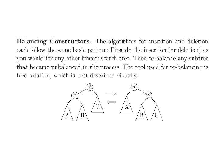
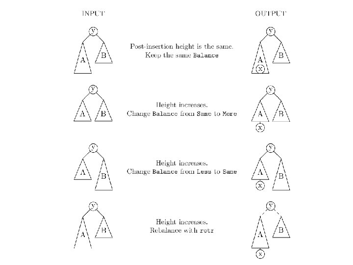
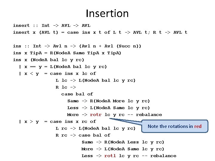
Insertion insert : : Int -> AVL insert x (AVL t) = case ins x t of L t -> AVL t; R t -> AVL t ins ins | | : : Int -> Avl n -> (Avl n + Avl (Succ n)) x Tip. A = R(Node. A Same Tip. A x Tip. A) x (Node. A bal lc y rc) x == y = L(Node. A bal lc y rc) x < y = case ins x lc of L lc -> L(Node. A bal lc y rc) R lc -> case bal of Same -> R(Node. A More lc y rc) Less -> L(Node. A Same lc y rc) More -> rotr lc y rc -- rebalance | x > y = case ins x rc of Note the rotations in red L rc -> L(Node. A bal lc y rc) R rc -> case bal of Same -> R(Node. A Less lc y rc) More -> L(Node. A Same lc y rc) Less -> rotl lc y rc -- rebalance

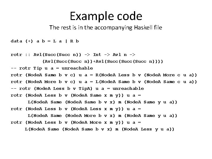
Example code The rest is in the accompanying Haskell file data (+) a b = L a | R b rotr : : Avl(Succ n)) -> Int -> Avl n -> (Avl(Succ n))+Avl(Succ(Succ n)))) -- rotr Tip u a = unreachable rotr (Node. A Same b v c) u a = R(Node. A Less b v (Node. A More c u a)) rotr (Node. A More b v c) u a = L(Node. A Same b v (Node. A Same c u a)) -- rotr (Node. A Less b v Tip. A) u a = unreachable rotr (Node. A Less b v (Node. A Same x m y)) u a = L(Node. A Same b v x) m (Node. A Same y u a)) rotr (Node. A Less b v (Node. A Less x m y)) u a = L(Node. A Same (Node. A More b v x) m (Node. A Same y u a)) rotr (Node. A Less b v (Node. A More x m y)) u a = L(Node. A Same b v x) m (Node. A Less y u a))

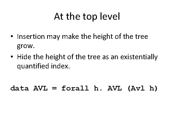
At the top level • Insertion may make the height of the tree grow. • Hide the height of the tree as an existentially quantified index. data AVL = forall h. AVL (Avl h)

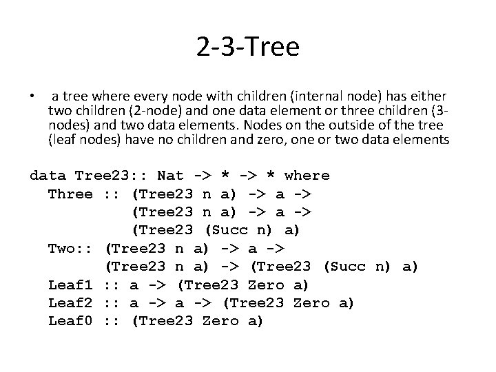
2 -3 -Tree • a tree where every node with children (internal node) has either two children (2 -node) and one data element or three children (3 nodes) and two data elements. Nodes on the outside of the tree (leaf nodes) have no children and zero, one or two data elements data Tree 23: : Nat -> * where Three : : (Tree 23 n a) -> a -> (Tree 23 (Succ n) a) Two: : (Tree 23 n a) -> a -> (Tree 23 n a) -> (Tree 23 (Succ n) a) Leaf 1 : : a -> (Tree 23 Zero a) Leaf 2 : : a -> (Tree 23 Zero a) Leaf 0 : : (Tree 23 Zero a)

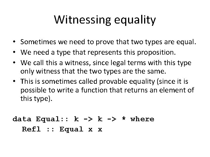
Witnessing equality • Sometimes we need to prove that two types are equal. • We need a type that represents this proposition. • We call this a witness, since legal terms with this type only witness that the two types are the same. • This is sometimes called provable equality (since it is possible to write a function that returns an element of this type). data Equal: : k -> * where Refl : : Equal x x

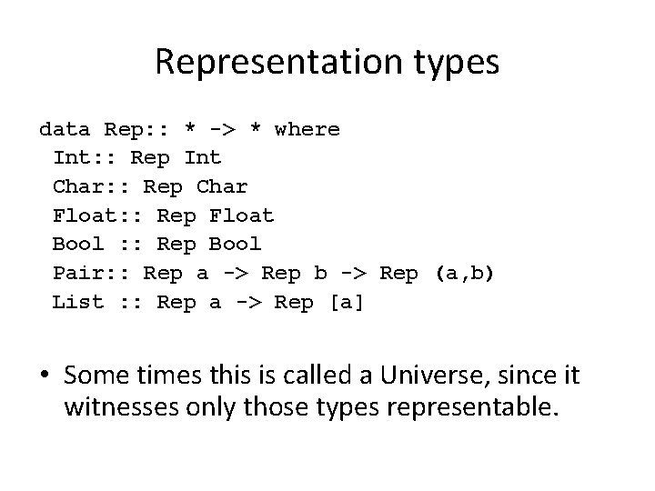
Representation types data Rep: : * -> * where Int: : Rep Int Char: : Rep Char Float: : Rep Float Bool : : Rep Bool Pair: : Rep a -> Rep b -> Rep (a, b) List : : Rep a -> Rep [a] • Some times this is called a Universe, since it witnesses only those types representable.

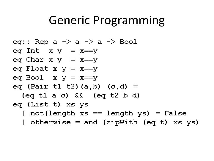
Generic Programming eq: : Rep a -> Bool eq Int x y = x==y eq Char x y = x==y eq Float x y = x==y eq Bool x y = x==y eq (Pair t 1 t 2)(a, b) (c, d) = (eq t 1 a c) && (eq t 2 b d) eq (List t) xs ys | not(length xs == length ys) = False | otherwise = and (zip. With (eq t) xs ys)

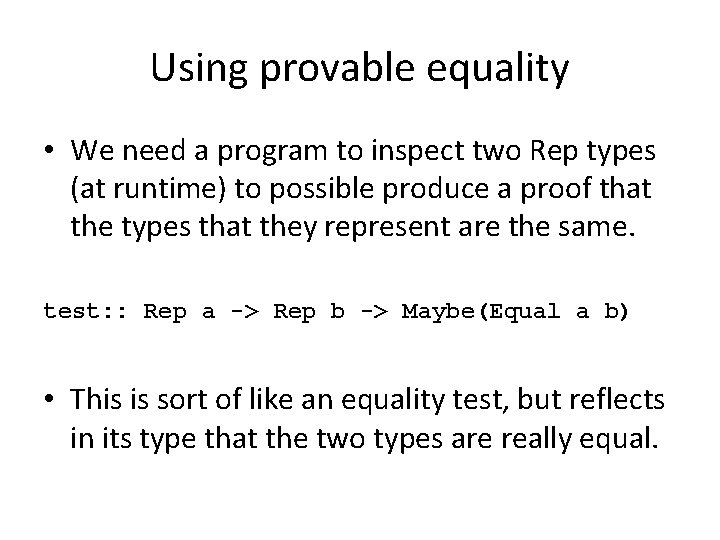
Using provable equality • We need a program to inspect two Rep types (at runtime) to possible produce a proof that the types that they represent are the same. test: : Rep a -> Rep b -> Maybe(Equal a b) • This is sort of like an equality test, but reflects in its type that the two types are really equal.

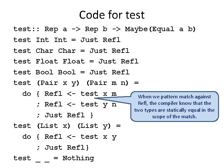
Code for test: : Rep a -> Rep b -> Maybe(Equal a b) test Int = Just Refl test Char = Just Refl test Float = Just Refl test Bool = Just Refl test (Pair x y) (Pair m n) = do { Refl <- test x m When we pattern match against Refl, the compiler know that the ; Refl <- test y n two types are statically equal in the ; Just Refl } scope of the match. test (List x) (List y) = do { Refl <- test x y ; Just Refl} test _ _ = Nothing

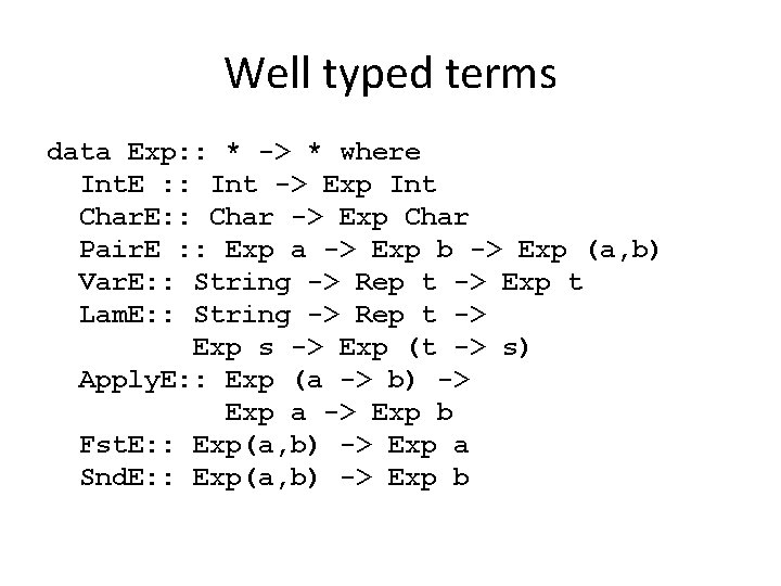
Well typed terms data Exp: : * -> * where Int. E : : Int -> Exp Int Char. E: : Char -> Exp Char Pair. E : : Exp a -> Exp b -> Exp (a, b) Var. E: : String -> Rep t -> Exp t Lam. E: : String -> Rep t -> Exp s -> Exp (t -> s) Apply. E: : Exp (a -> b) -> Exp a -> Exp b Fst. E: : Exp(a, b) -> Exp a Snd. E: : Exp(a, b) -> Exp b

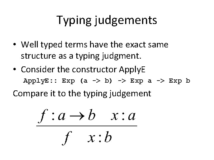
Typing judgements • Well typed terms have the exact same structure as a typing judgment. • Consider the constructor Apply. E: : Exp (a -> b) -> Exp a -> Exp b Compare it to the typing judgement

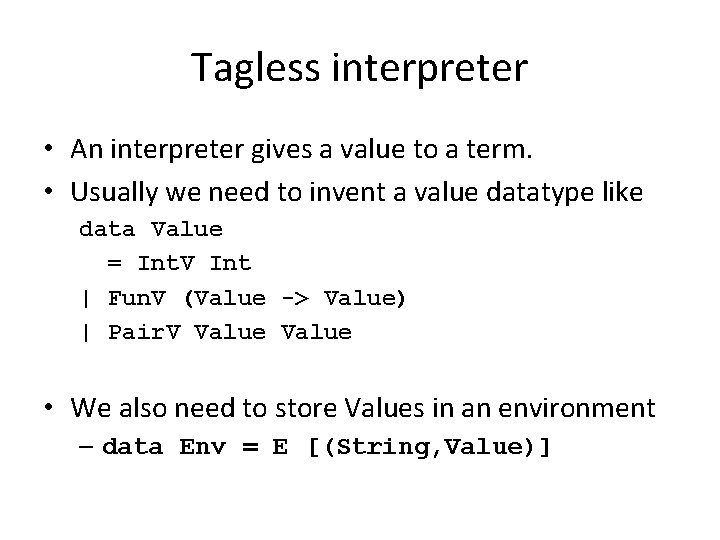
Tagless interpreter • An interpreter gives a value to a term. • Usually we need to invent a value datatype like data Value = Int. V Int | Fun. V (Value -> Value) | Pair. V Value • We also need to store Values in an environment – data Env = E [(String, Value)]

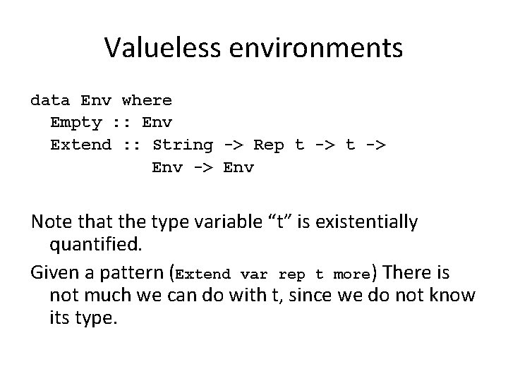
Valueless environments data Env where Empty : : Env Extend : : String -> Rep t -> Env Note that the type variable “t” is existentially quantified. Given a pattern (Extend var rep t more) There is not much we can do with t, since we do not know its type.

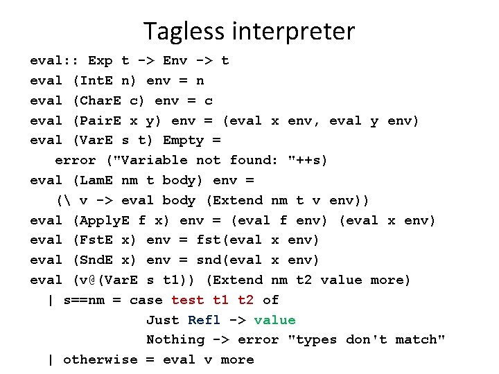
Tagless interpreter eval: : Exp t -> Env -> t eval (Int. E n) env = n eval (Char. E c) env = c eval (Pair. E x y) env = (eval x env, eval y env) eval (Var. E s t) Empty = error ("Variable not found: "++s) eval (Lam. E nm t body) env = ( v -> eval body (Extend nm t v env)) eval (Apply. E f x) env = (eval f env) (eval x env) eval (Fst. E x) env = fst(eval x env) eval (Snd. E x) env = snd(eval x env) eval (v@(Var. E s t 1)) (Extend nm t 2 value more) | s==nm = case test t 1 t 2 of Just Refl -> value Nothing -> error "types don't match" | otherwise = eval v more

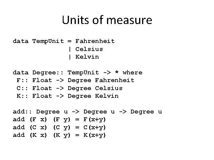
Units of measure data Temp. Unit = Fahrenheit | Celsius | Kelvin data F: : C: : K: : Degree: : Float -> add: : Degree add (F x) (F add (C x) (C add (K x) (K Temp. Unit -> * where Degree Fahrenheit Degree Celsius Degree Kelvin u -> y) = Degree u -> Degree u F(x+y) C(x+y) K(x+y)

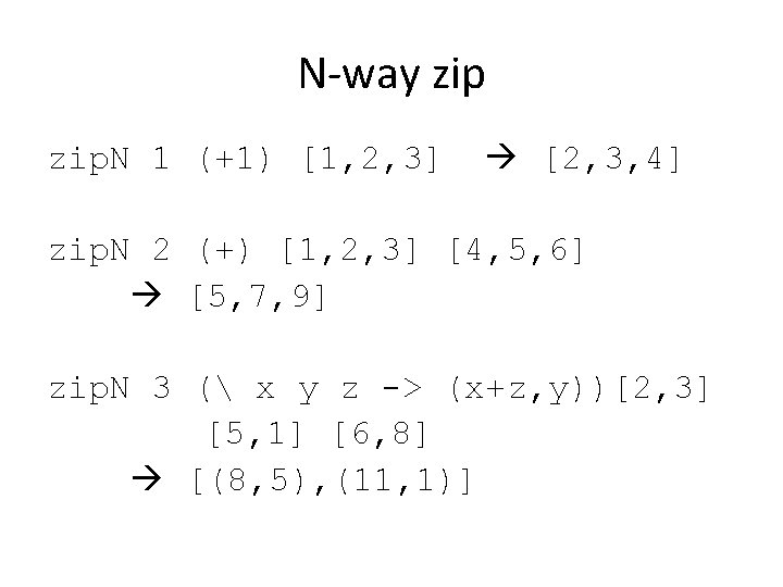
N-way zip. N 1 (+1) [1, 2, 3] [2, 3, 4] zip. N 2 (+) [1, 2, 3] [4, 5, 6] [5, 7, 9] zip. N 3 ( x y z -> (x+z, y))[2, 3] [5, 1] [6, 8] [(8, 5), (11, 1)]

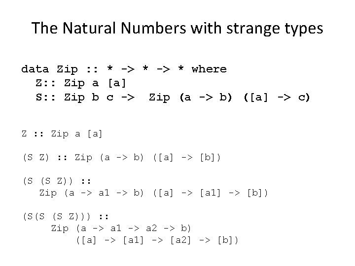
The Natural Numbers with strange types data Zip : : * -> * where Z: : Zip a [a] S: : Zip b c -> Zip (a -> b) ([a] -> c) Z : : Zip a [a] (S Z) : : Zip (a -> b) ([a] -> [b]) (S (S Z)) : : Zip (a -> a 1 -> b) ([a] -> [a 1] -> [b]) (S(S (S Z))) : : Zip (a -> a 1 -> a 2 -> b) ([a] -> [a 1] -> [a 2] -> [b])

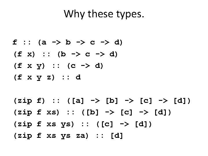
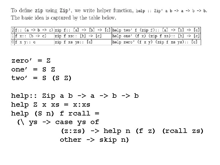
zero’ = Z one’ = S Z two’ = S (S Z) help: : Zip a b -> a -> b help Z x xs = x: xs help (S n) f rcall = ( ys -> case ys of (z: zs) -> help n (f z) (rcall zs) other -> skip n)

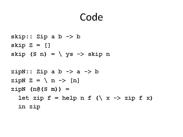
Code skip: : Zip a b -> b skip Z = [] skip (S n) = ys -> skip n zip. N: : Zip a b -> a -> b zip. N Z = n -> [n] zip. N (n@(S m)) = let zip f = help n f ( x -> zip f x) in zip